
基于高分辨ROMS模式的黑潮延伸体次中尺度涡各向异性分析
|
周霄雯(1994—), 女, 山东省烟台市人, 硕士研究生, 从事中小尺度海洋过程研究。E-mail: |
收稿日期: 2019-06-17
要求修回日期: 2019-12-13
网络出版日期: 2020-05-19
基金资助
国家重点研发计划(2017YFA0604104)
热带海洋环境国家重点实验室(中科院南海海洋研究所)开放课题(LTO1907)
中国博士后基金(2018M642148)
江苏省博士后科研资助计划(2018K149C)
国家自然科学基金(41776040)
青岛海洋科学与技术试点国家实验室OCFL功能实验室开放课题(201804)
版权
Anisotropy of submesoscale eddy in Kuroshio Extension based on high resolution ROMS output analysis
Received date: 2019-06-17
Request revised date: 2019-12-13
Online published: 2020-05-19
Supported by
The National Key Research and Development Program of China(2017YFA0604104)
Opening Foundation of State Key Laboratory of Tropical Oceanography(South China Sea Institute of Oceanology, Chinese Academy of Sciences)(LTO1907)
Chinese Postdoctoral Foundation(2018M642148)
Jiangsu Planned Projects for Postdoctoral Research Funds(2018K149C)
National Natural Science Foundation of China(41776040)
Opening of OCFL Functional Laboratory of Qingdao Pilot National Laboratory of Marine Science and Technology(201804)
Copyright
次中尺度过程的水平空间尺度约为0.1~10km, 时间尺度约为1天, 里查森数和罗斯贝数为0(1), 能有效地从中尺度环流中汲取能量向小尺度湍流串级, 并对上层海洋物质的垂向交换有着重要影响。本文基于水平分辨率为~500m的高分辨率ROMS(regional ocean modeling system)数值模拟结果, 采用方差椭圆方法, 评估了黑潮延伸体海域上层海洋次中尺度涡旋的各向异性特征, 并探讨了涡旋各向异性值的大小与次中尺度过程特征参数的相关性。研究结果表明, 黑潮延伸体主轴强流区域的次中尺度涡旋各向异性值明显小于两侧海域, 主轴区域的次中尺度涡旋特征明显强于流轴两侧海域, 各向异性值与次中尺度过程的强弱有着较为显著的负相关关系, 表明次中尺度过程具有较小的各向异性特征(更趋各向同性)。方差椭圆表征了涡与平均流相互作用过程中的能量反馈机制, 较大的各向同性特征意味着动能更趋正向串级。
周霄雯 , 曹海锦 , 经志友 , 廖光洪 . 基于高分辨ROMS模式的黑潮延伸体次中尺度涡各向异性分析[J]. 热带海洋学报, 2020 , 39(3) : 10 -18 . DOI: 10.11978/2019056
Submesoscale eddies have smaller Richardson number and larger Rossby number, with horizontal scales between 0.1 and 10 km and time scale of ~0(1 day). They act to extract energy from the mesoscale circulation, drive forward energy cascade to the smaller scale turbulence and meanwhile contribute to the vertical flux of what in the upper ocean. In this study, anisotropy of submesoscale eddies in the Kuroshio Extension in a high-resolution simulation (∆x≈500m) by the regional ocean modeling system (ROMS) is evaluated using the nummular variance ellipse method. A correlation between eddy anisotropy and submesoscale features is also analyzed. The results show that the submesoscale eddies, as well as the anisotropy, near the flow stream get intensified compared to those in the flanks. The isotropic ratio is well correlated with the strength of submesoscale processes, suggesting that the submesoscale processes tend to be isotropic. The nummular variance ellipse, known as the feedback of eddies to mean flow, may implies forward cascade of kinetic energy.
Key words: submesoscale eddy; Kuroshio Extension; eddy anisotropy; energy cascade; upper ocean
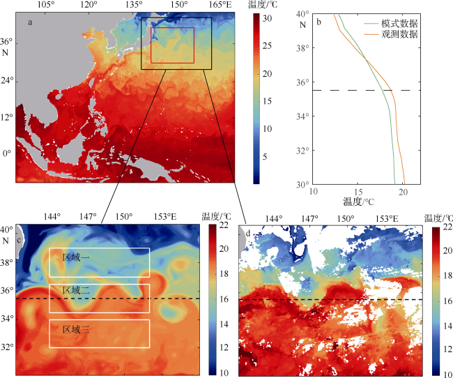
图1 ROMS模式数据和相应区域的MODIS卫星数据的温度分布及其对比a. 模式模拟区域的水平分辨率为7.5km的表层温度场(黑色方框区域和红色方框区域分别代表网格分辨率为∆x≈1.5km和∆x≈500m的嵌套区域); b. 模式数据与MODIS卫星数据温度(纬向平均)随纬度的分布; c. 模式模拟区域的水平分辨率为500m的表层温度场(白色方框所示的三个子区域是为方便后文分析对比黑潮延伸体流轴区域与其他区域的差别); d. MODIS卫星数据的表层温度场。图中模式温度场均为4月21日至5月4日8d平均的数据, 卫星温度场为2018年4月21日至5月4日8d平均的数据 Fig. 1 Temperature distribution and comparison between ROMS model data and MODIS satellite data in corresponding domain. a) Surface temperature field of model domain with horizontal resolution of 7.5 km (the black box area and the red box area respectively represent the nested areas with grid resolution of ∆x≈1.5km and ∆x≈500m); b) temperature (zonally averaged) distribution with latitude in the model data and MODIS satellite data; c) surface temperature field of model domain with horizontal resolution of 500 m (the three sub-domains shown in the white box are for the convenience of later analysis and comparison of the differences between the Kuroshio extensional flow axis domain and other domains); d) surface temperature field from MODIS satellite data. The temperature field in the model is averaged for eight days from April 21 to May 4, and satellite temperature field is averaged for eight days from April 21 to May 4, 2018. |
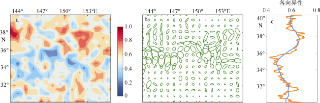
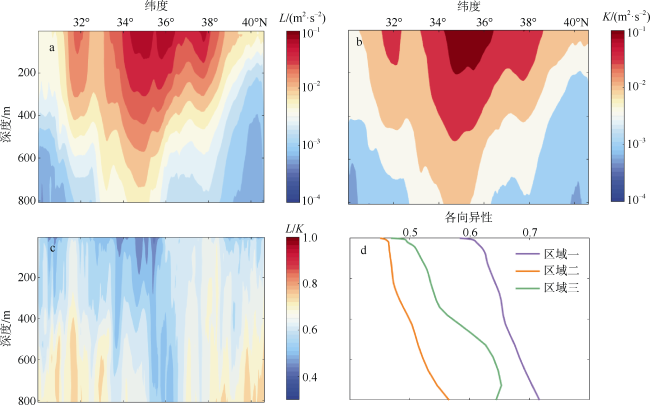
图4 各向异性值(L/K)的表层分布a. 水平分辨率为0.5°的各向异性值; b. 用椭圆表示的各向异性值; c. 纬向平均后的各向异性值(橙色线为各向异性值, 蓝色线为拟合后的曲线) Fig. 4 Surface distribution of anisotropy. a) Anisotropy with horizontal resolution of 0.5°; b) anisotropy represented by ellipse; c) latitudinally averaged anisotropy (the orange line is the anisotropy profile, and the blue line is the fitted profile) |
表1 三个区域的K、L和L/K的平均值Tab. 1 Mean K, L and L/K in three regions |
| K/(m2·s-2) | L/(m2·s-2) | L/K | |
|---|---|---|---|
| 区域一 | 0.028 | 0.017 | 0.6 |
| 区域二 | 0.096 | 0.038 | 0.4 |
| 区域三 | 0.025 | 0.015 | 0.6 |
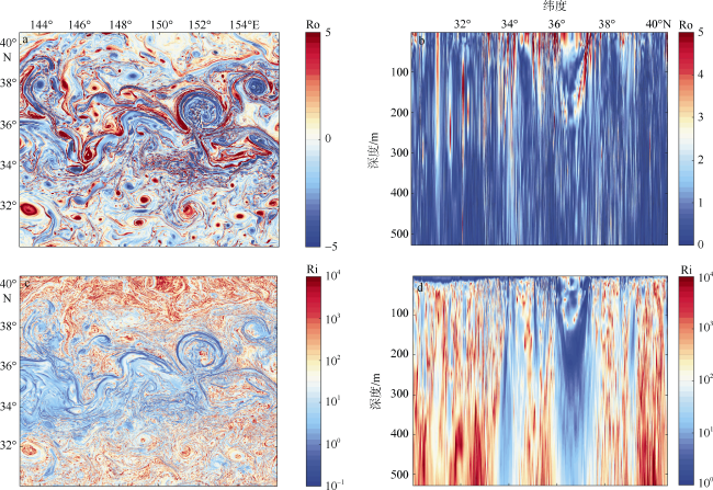
图6 罗斯贝数和里查森数的分布a. 表层罗斯贝数的水平分布; b. 罗斯贝数(绝对值)的垂向分布; c. 表层里查森数的水平分布; d. 里查森数(绝对值)的垂向分布。时间为4月28日12时 Fig. 6 Distributions of Rossby number and Richardson number. a) Horizontal distribution of surface Rossby number; b) vertical distribution of Rossby number (absolute value); c) horizontal distribution of surface Richardson number; d) vertical distribution of Richardson number (absolute value). Time: 12:00 on April 28 |
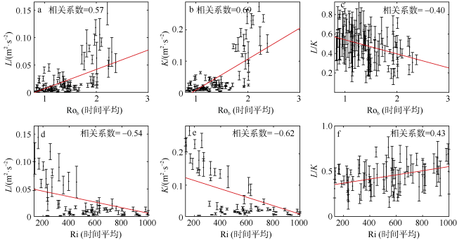
图8 L、K以及L/K值与罗斯贝数和里查森数的相关关系a. L与斜压罗斯贝数的相关关系 ; b. K与斜压罗斯贝数的相关关系; c. L/K与斜压罗斯贝数的相关关系; d. L与里查森数的相关关系; e. K与里查森数的相关关系; f. L/K与里查森数的相关关系 Fig. 8 Correlation with Rossby number and Richardson number. a) Correlation between L and baroclinic Rossby number; b) correlation between K and baroclinic Rossby number; c) correlation between L/K and baroclinic Rossby number; d) correlation between L and Richardson number; e) correlation between K and Richardson number; f) correlation between L/K and Richardson number |
| 1 |
|
| 2 |
|
| 3 |
|
| 4 |
|
| 5 |
|
| 6 |
|
| 7 |
|
| 8 |
|
| 9 |
|
| 10 |
|
/
| 〈 |
|
〉 |
