
利用海洋温度剖面与海表盐度反演盐度剖面方法研究
|
何子康(1996—), 硕士研究生, 主要从事物理海洋学研究。email: |
Copy editor: 林强
收稿日期: 2020-12-01
修回日期: 2021-03-05
网络出版日期: 2021-03-15
基金资助
国家自然科学基金(4177060056)
版权
Reconstructing salinity profile using temperature profile and sea surface salinity
Copy editor: LIN Qiang
Received date: 2020-12-01
Revised date: 2021-03-05
Online published: 2021-03-15
Supported by
National Natural Science Foundation of China(4177060056)
Copyright
为解决海洋中大量观测数据只含有温度剖面而缺乏盐度观测的问题, 基于历史观测的温盐剖面资料, 考虑到盐度卫星数据的发展, 采用回归分析方法, 在孟加拉湾建立了盐度与温度、经纬度、表层盐度的关系, 并对不同反演方法的反演结果进行检验评估。结果发现, 在不引入海表盐度(sea surface salinity, SSS)时, 最佳反演模型是温度、温度的二次项与经纬度确定的回归模型, 而SSS的引入则可以进一步优化反演结果。将反演结果与观测结果进行对比, 显示用反演的盐度剖面计算的比容海面高度误差超过2cm, 而引入SSS后的误差低于1.5cm。SSS的引入能够较为真实地反映海洋盐度场的垂直结构和内部变化特征, 既能够捕捉到对上混合层有重要影响的SSS信号, 又能够反映盐度在跃层上的季节内变化以及盐度障碍层的季节变化。水团分析显示, 与气候态相比, 盐度反演结果可以更好地表征海洋上层水团的变化特征。
何子康 , 王喜冬 , 陈志强 , 范开桂 . 利用海洋温度剖面与海表盐度反演盐度剖面方法研究[J]. 热带海洋学报, 2021 , 40(6) : 41 -51 . DOI: 10.11978/2020141
A large number of marine observations contain only temperature profiles, but not salinity profiles that are important for understanding ocean dynamics. To construct salinity profiles, we use regression analysis methods to establish relationship of ocean salinity with historical ocean temperature, longitude, latitude, and satellite-based sea surface salinity (SSS) in the Bay of Bengal. The results of different inversion methods are then tested and evaluated. We find that without introducing SSS, the best reconstruct model is using temperature, namely, using the secondary items of temperature with longitude and latitude to determine the regression model. However, the introduction of SSS can further improve the inversion results. By comparing the reconstructions with the observations, we show that the steric height error calculated by the salinity profile inversion is more than 2.0 cm, while the error calculated after introducing SSS is less than 1.5 cm. The introduction of SSS can truly reflect the vertical structure and internal variation characteristics of ocean salinity profile. It can not only capture the SSS signal that has an important influence on the upper mixing layer, but also reflect the seasonal change of salinity on the thermocline and the seasonal change of the barrier layer. The inversion results are compared with the climatology, and the observed water mass is analyzed, showing that compared with the climatology, the inversion can better represent the variation characteristics of the surface water mass. However, below the mixing layer, there is no significant difference between the inversion and climatology.
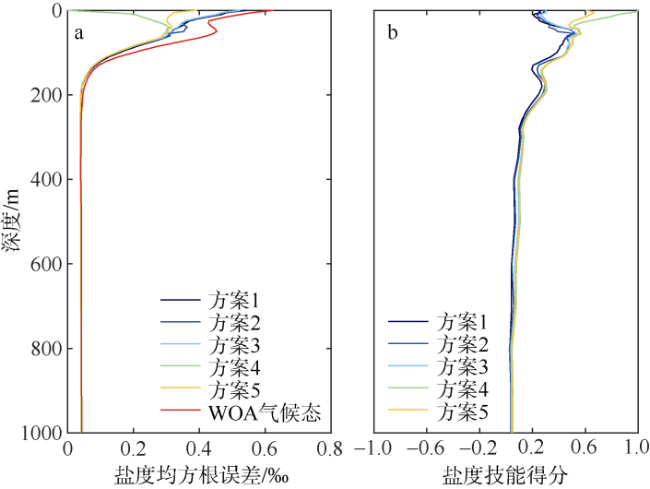
图3 4种不同反演盐度剖面方案中WOA气候态与实测资料之间的均方根误差随水深的变化(a)以及4种不同反演盐度剖面方案的技能得分(b)Fig. 3 RMSEs between WOA13 salinity and each of the four salinity reconstructions, showing in situ profiles (a) and skill scores of the four schemes (b) |
表1 不同方案垂向平均均方根误差Tab. 1 Mean RMSEs of different schemes |
| 实验方案 | 盐度垂向平均均方根误差/‰ |
|---|---|
| 方案1 | 0.2011 |
| 方案2 | 0.1993 |
| 方案3 | 0.1946 |
| 方案4 | 0.1341 |
| 方案5 | 0.1682 |
| WOA13气候态 | 0.2451 |
表2 不同方案垂向平均均方根误差Tab. 2 RMSEs of different schemes |
| 实验方案 | 均方根误差/cm |
|---|---|
| 方案1 | 2.37 |
| 方案2 | 2.16 |
| 方案3 | 2.32 |
| 方案4 | 1.48 |
| 方案5 | 1.28 |
| WOA13气候态 | 2.98 |
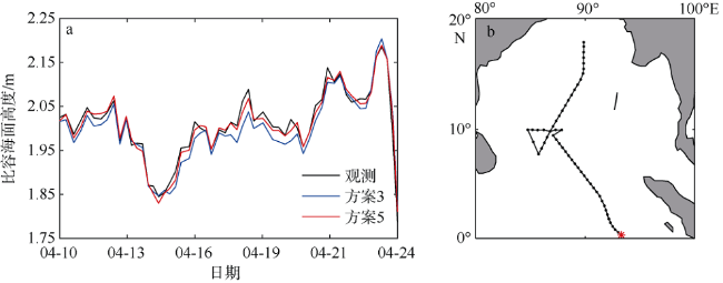
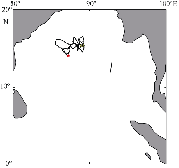
图4 不同方案反演盐度剖面计算的比容海面高度(a)和CTD航次轨迹(b)b中红点代表船的起始位置。该图基于国家测绘地理信息局标准地图服务网站下载的审图号为GS(2020)4392号的标准地图制作。 Fig. 4 Steric height of salinity profile reconstruction calculated using different schemes (a) and the cruise track of CTD (b), and the red star represents the start of the cruise |
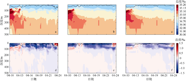
图5 观测盐度断面及其重构结果a. 实测盐度断面; b.卫星观测作为表层盐度引入的方案5反演盐度断面; c.方案3反演盐度断面; d. 实测盐度异常断面; e. 方案5反演盐度断面; f. 方案3反演盐度异常断面。图中黑线表示混合层深度 Fig. 5 Salinity profile results. (a) Observed salinity profiles; (b) scheme 5 inversion salinity profiles using satellite SSS; (c) scheme 3 inversion of salinity profiles; (d) measured salinity abnormal profiles; (e) inversion of salinity anomaly profiles using scheme 4; and (f) inversion of salinity anomaly profiles using scheme 3. The black curve indicates mixed-layer depth |
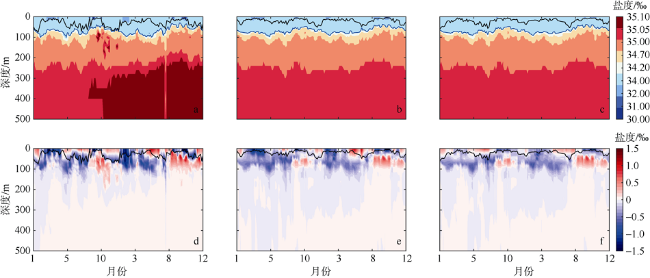
图7 2016—2017年间观测盐度断面及其重构结果a. 实测盐度断面; b. 卫星观测作为表层盐度引入的方案4反演盐度断面; c. 方案3反演盐度断面; d. 实测盐度异常断面; e. 卫星观测作为表层盐度引入的方案4反演盐度断面; f. 方案3反演盐度异常断面;图中黑线表示混合层深度; a—c图中的蓝色实心曲线代表盐度34.2‰的等值线 Fig. 7 Results of observed salinity profiles and reconstruction during 2016-2017. (a) Observed salinity profiles; (b) reconstructed salinity profiles by scheme 4, using satellite SSS; (c) reconstructed salinity profiles by scheme 3; (d) observed salinity anomaly profiles; (e) reconstructed salinity anomaly profiles using scheme 4 and satellite SSS; (f) WOA13 climatology salinity anomaly profiles. The black curve is the mixed-layer depth, and the blue curve in (a-c) represents the depth of salinity isoline 34.2‰ |
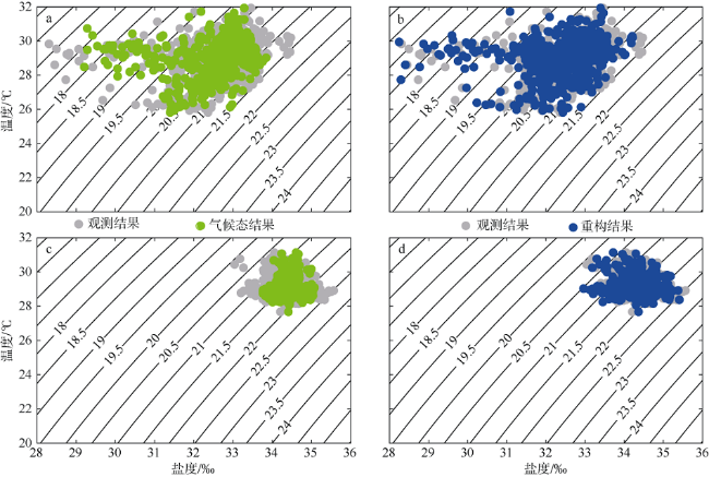
图9 0m处孟加拉湾WOA气候态结果和反演结果与观测结果的对比a. WOA气候态结果与观测结果对比; b.反演结果与观测结果对比; c. 孟加拉湾赤道WOA气候态结果与观测结果对比; d. 孟加拉湾赤道反演结果与观测结果对比。图中等值线代表位势密度的超量 Fig. 9 Comparison between WOA climatology and reconstruction results with observations in the Bay of Bengal at 0m. (a) Comparison of WOA climatology and observations; (b) comparison of reconstruction and observations; (c) comparison of observations and WOA climatology on the equator in the Bay of Bengal; and (d) comparison of observations and reconstruction on the equator in the Bay of Bengal. |
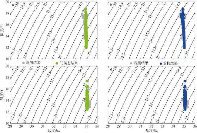
图10 200m处孟加拉湾WOA气候态结果和反演结果与观测结果的对比Fig. 10 Comparison between WOA climatology and reconstruction results with observations in the Bay of Bengal at 200 m |
| [1] |
宣莉莉, 邱云, 许金电, 等, 2015. 孟加拉湾与赤道东印度洋水交换的季节变化特征[J]. 热带海洋学报, 34(6):26-34.
|
| [2] |
张玉红, 杜岩, 徐海明, 2012. 赤道印度洋中部断面东西水交换的季节变化及其区域差异[J]. 海洋学报(中文版), 34(2):30-38.
|
| [3] |
|
| [4] |
|
| [5] |
|
| [6] |
|
| [7] |
|
| [8] |
|
| [9] |
|
| [10] |
|
| [11] |
|
| [12] |
|
| [13] |
|
| [14] |
|
| [15] |
|
| [16] |
|
| [17] |
|
| [18] |
|
| [19] |
|
| [20] |
|
| [21] |
|
| [22] |
|
| [23] |
|
| [24] |
|
/
| 〈 |
|
〉 |
