
海洋中示踪物等值线的分形长度及其与混合效率的关系*
*感谢南海海洋研究所的高性能计算中心为本文数值模拟提供的技术支持。
|
钱钰坤(1983—), 男, 广西柳州市人, 博士, 从事海洋数值模拟与混合参数化研究。email: |
Editor: Cuici
Copy editor: 孙翠慈SUN
收稿日期: 2023-05-12
修回日期: 2023-06-08
网络出版日期: 2023-06-01
基金资助
国家重点研发项目(2022YFC3105004)
国家自然科学基金项目(41976023)
国家自然科学基金项目(41931182)
国家自然科学基金项目(42106008)
国家自然科学基金项目(42376028)
热带海洋环境国家重点实验室自主研究项目(LTOZZ2102)
热带海洋环境国家重点实验室开放课题(LTO2107)
Fractal lengths of tracer contours in the ocean and its relationship with mixing efficiency
Editor: Cuici
Received date: 2023-05-12
Revised date: 2023-06-08
Online published: 2023-06-01
Supported by
National Key Research and Development Program of China(2022YFC3105004)
National Natural Science Foundation of China(41976023)
National Natural Science Foundation of China(41931182)
National Natural Science Foundation of China(42106008)
National Natural Science Foundation of China(42376028)
Independent Research Project Program of State Key Laboratory of Tropical Oceanography(LTOZZ2102)
Open Project of the State Key Laboratory of Tropical Oceanography(LTO2107)
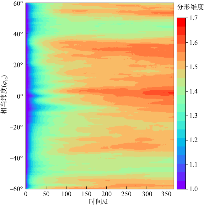
涡致混合扩散是物理海洋研究中的热点和难点问题。本文基于“有效扩散”理论, 研究示踪物等值线在海表地转湍流的多尺度搅拌作用下, 发生拉伸、扭曲、变形、折叠等改变其几何拓扑结构的现象, 并探讨了等值线分形长度的变化与混合效率的关系。研究结果表明, 在地转流场的搅拌下, 示踪物的等值线会被迅速拉长, 并产生丰富的精细结构。这种分形式的增长可达原长度的10~20倍, 是混合效率提高的主要原因; 而涡丝和锋面伴随的梯度增强虽然也有贡献, 但为次要因素。另一方面, 在示踪物模拟过程中, 小尺度扩散会通过不可逆混合对示踪物进行均匀化, 从而抹平等值线的精细结构, 抑制等值线的增长, 限制混合效率的提高。基于“数盒子”算法计算了等值线的分形维度, 其数值在1.4到1.6之间, 介于一维和二维之间。但由于地转湍流数据分辨率的限制, 无法考虑更小尺度(次中尺度过程)的搅拌作用, 可能低估了等值线的分形长度和混合效率。本研究将海洋混合与等值线几何特征联系了起来, 初步得到了分形长度和混合效率两者的经验关系式, 未来可以利用图像识别等成熟遥感技术将海洋示踪物等值线的几何特征直接转换为混合效率, 为诊断分析海洋混合及其参数化提供了一种新的思路。
钱钰坤 , 刘统亚 , 张华 , 彭世球 . 海洋中示踪物等值线的分形长度及其与混合效率的关系*[J]. 热带海洋学报, 2024 , 43(1) : 1 -15 . DOI: 10.11978/2023020
Quantifying eddy mixing in the ocean is a hot and tough problem in the area of physical oceanography. Based on the theory of effective diffusivity, the present study investigated the stirring effects of geostrophic turbulence that led to stretching, distorting, deforming, and folding of tracer contours. These changes are then related to the efficiency of turbulent mixing. Results show that under the stirring effect of geostrophic turbulence, the length of tracer contour can be quickly elongated and fine-scale tracer filaments and fronts are also generated. This fractal elongation of tracer contour, about 10~20 times longer than the original length, is the dominant contributor to the mixing efficiency, whereas the gradient enhancement associated with filament and front generations only plays a secondary role. On the other hand, fine-scale features are smoothed out by small-scale diffusivity which eventually suppresses the increase of contour length and the generation of tracer filaments. This imposes an upper bound of the mixing efficiency when the stirring and smoothing effects are in a dynamical balance. Through a ‘box-counting’ method, the fractal dimension of tracer contour is also found between 1.4~1.6, indicating a geometric dimension lies somewhere between 1D and 2D. Due to the limitation of data resolution, contour length and thus mixing efficiency may be underestimated. Finally, the present study made an empirical relation between the fractal dimension and mixing efficiency, providing an opportunity for estimating mixing efficiency through a well-developed pattern recognition technique in remote sensing, and a new way of diagnosing ocean mixing and its parameterization.
图1 示踪物等值线长度与混合效率关系示意图a. 等值线为球面上最短曲线时的分布(为同心圆或纬圈线), 此时混合效率最低; b. 气候态(欧拉时间平均)等值线分布; c. 瞬时等值线分布图, 此时其混合效率相比(a)和(b)具有数量级的提高; 三个状态中等值线包围的面积相等; 审图号为GS (2016)1665 Fig.1 Schematic illustration of the relation between contour length of a tracer and mixing efficiency. (a) Minimum possible contour length on a sphere (latitude circles) which is at the lowest mixing efficiency; (b) smooth climatological contour through a Eulerian time mean; (c) instantaneous wavy contour distribution in which mixing efficiency is greatly enhanced. Note that the areas between any two contours are the same for each panel |
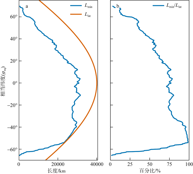
图3 等值线最短长度${{L}_{\text{min}}}$(km, 蓝线)和纬圈总长度(km, 橙线)(a)以及${{L}_{\text{min}}}$占纬圈总长度的百分比(b)Fig. 3 (a) Minimum possible length ${{L}_{\text{min}}}$ (km, blue) and total length of latitudinal circle (km, orange), and (b) the ratio of ${{L}_{\text{min}}}$ to the total length of latitudinal circle |
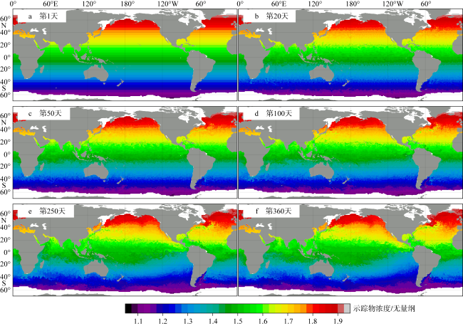
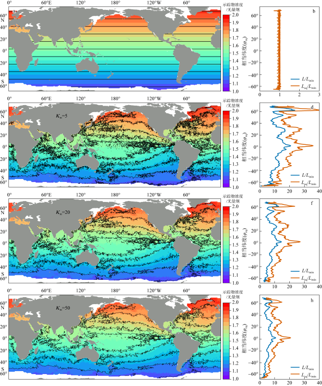
图4 示踪物水平分布及等值线长度a. 初始时刻的示踪物水平分布; c、 e、 g: 分别为用小尺度扩散系数${{\kappa }_{m}}=5$、20、50 m2·s−1积分一年后的为示踪物的水平分布, 黑实线为任意选取的一组等值线用于展示其拓扑细节; b、d、 f、 h: 等值线长度L(蓝色)和相当长度${{L}_{\text{eq}}}$(橙色), 两者均用${{L}_{\text{min}}}$做单位进行无量纲化; 图中审图号为GS(2016)1665 Fig. 4 Tracer horizontal distribution and its contour length L and equivalent length ${{L}_{\text{eq}}}$. Left columns are tracer distributions with several contours highlighted. Right columns are contour lengths normalized by ${{L}_{\text{min}}}$(b, d, f, h). The first row is the results at first day (a) and the last three rows are results after 1-yr integration with small-scale diffusivity ${{\kappa }_{\text{m}}}=$ 5(c), 20(e), 50 m2·s-1(g) |
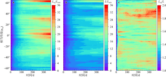
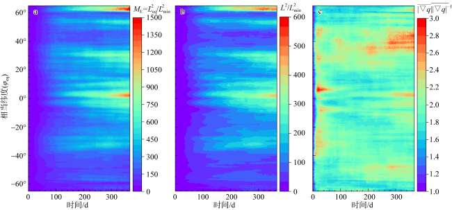
图6 (a)混合效率${{M}_{\text{E}}}$, (b)等值线增长因子${{L}^{2}}/L_{\text{min}}^{2}$, (c)梯度因子$\overline{\left| \nabla q \right|}\overline{{{\left| \nabla q \right|}^{-1}}}$Fig. 6 Temporal evolutions of (a) mixing efficiency ${{M}_{\text{E}}}$ (b) perimeter length factor ${{L}^{2}}/L_{\text{min}}^{2}$, and (c) gradient factor $\overline{\left| \nabla q \right|}\overline{{{\left| \nabla q \right|}^{-1}}}$ |
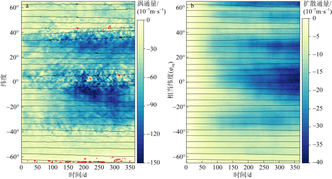
图7 基于欧拉纬向平均的经向涡动通量和沿等值线平均的扩散通量对比图a. 经向涡动通量${{\overline{v'q'}}^{X}}$(10-5, 填色)和${{\bar{q}}^{X}}$(等值线), 其中${{\overline{\left( \cdot \right)}}^{X}}$表示欧拉纬向平均, ${{\left( \text{ }\!\!\cdot\!\!\text{ } \right)}^{\prime }}$表示对应的距平; b. 基于等值线平均的扩散通量${{K}_{\text{eff}}}\partial q/\partial {{\varphi }_{\text{eq}}}/a$(10-5, 填色)和$q\left( t,{{\varphi }_{\text{eq}}} \right)$(等值线); 其中红色等值线为通量的0等值线 Fig. 7 Comparison of Eulerian zonal mean eddy flux and along-contour mean diffusive flux. (a) Eddy tracer flux ${{\overline{v'q'}}^{X}}$ (10-5 color shadings) and ${{\bar{q}}^{X}}$ (contours) based on Eulerian zonal mean ${{\overline{\left( \text{ }\!\!\cdot\!\!\text{ } \right)}}^{X}}$; (b) diffusive flux ${{K}_{\text{eff}}}\partial q/\partial {{\varphi }_{\text{eq}}}/a$ (10-5) and $q\left( t,{{\varphi }_{\text{eq}}} \right)$ based on the along-contour mean. Red lines indicate zero-flux contour |
图8 示踪物浓度(无量纲)的水平分布(a、 c、 e、 g)及等值线长度(b、 d、 f、 h, 以${{L}_{\text{min}}}$为单位)第一行到第四行分别是积分1、20、100、365天后的结果。等值线长度采用了“数盒子”方法, 展示了8个网格距做尺子度量得到的结果。审图号为GS(2016)1665 Fig. 8 Tracer distributions at different timesteps (a, c, e, g) and contour lengths normalized by ${{L}_{\text{min}}}$(b, d, f, h). Row one to row four show the results of integration after 1, 20, 100, and 365 days. Contour lengths are calculated using ‘box-counting’ method with 8 grid boxes |
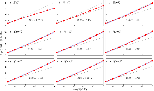
图9 相当纬度53.3°S对应的等值线长度(m)与网格分辨率(m)的对数关系从(a)到(i)分别为第0、10、50、100、150、200、250、300、350天的结果, 其中拟合斜率标注在各个子图内, 紫色阴影为95%拟合置信区间, 两条虚线分别是研究时段内最大和最小拟合斜率的曲线 Fig. 9 Contour length (m) against grid resolution (m) on a log-log plot for the equivalent latitude of 53.3°S. Panels (a) to (i) are results at 0, 10, 50, 100, 150, 200, 250, 300, and 350 days, respectively. Linear-fit slopes are indicated in each panel. Purple shadings indicate 95% confidence intervals for the linear fit. Two dash lines are the fitted lines with maximum and minimum slopes during the time range of interest |
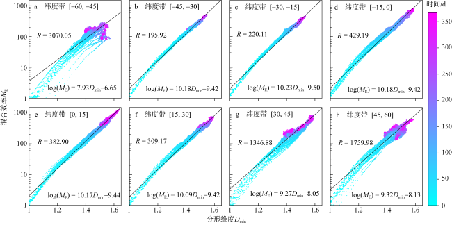
图11 分形维度(Dmin)与混合效率(ME)的散点关系图从(a)到(h)分别为不同纬圈范围的结果。颜色表示散点的时刻(天); 图中黑线为最小二乘拟合的直线, 拟合残差R以及拟合的线性方程分别标注在各个子图上 Fig. 11 Scatter plot of fractal dimension ${{D}_{\text{min}}}$ and mixing efficiency ${{M}_{\text{E}}}$. Panels (a) to (i) are results over different latitude bands. Colors indicates the time (day) relative to the first day. The black lines indicate a least-square linear fit, with residual R and the fitted equation labeled in each panel |
表1 |
| 纬度范围 | a±stderr | b±stderr | R |
|---|---|---|---|
| 60°S—45°S | 7.93±0.05 | −6.65±0.07 | 3070.05 |
| 45°S—30°S | 10.18±0.01 | −9.42±0.01 | 195.92 |
| 30°S—15°S | 10.23±0.01 | −9.50±0.01 | 220.11 |
| 15°S—0° | 10.18±0.01 | −9.42±0.02 | 429.19 |
| 0°—15°N | 10.17±0.01 | −9.44±0.02 | 382.90 |
| 15°N—30°N | 10.09±0.01 | −9.42±0.02 | 309.17 |
| 30°N—45°N | 9.27±0.02 | −8.05±0.04 | 1346.88 |
| 45°N—60°N | 9.32±0.03 | −8.13±0.04 | 1759.98 |
注: a、b分别为(13)式中的拟合斜率和截距, R为总残差, stderr为标准误差 | |
Notes:a, b: fitted slope and intercept in Eq. (13), R: total residual of the fit, stderr is standard error |
| [1] |
付昱华, 2000. 变换形成的分形与海洋环境数据分析预测[J]. 海洋通报, 19(1): 79-88.
|
| [2] |
黄真理, 2000. 湍流的分形特征[J]. 力学进展, 30(4): 581-596.
|
| [3] |
雷玺, 2015. 多重分形在海洋波高数据分析中的应用[D]. 青岛: 中国海洋大学.
|
| [4] |
刘式达, 付遵涛, 刘式适, 2014. 间歇湍流的分形特征——分数维及分数阶导数的应用[J]. 地球物理学报, 57(9): 2751-2755.
|
| [5] |
沈学会, 陈举华, 2005. 分形与混沌理论在湍流研究中的应用[J]. 河南科技大学学报(自然科学版), 26(1): 27-30.
|
| [6] |
田纪伟, 曹露洁, 楼顺里, 1996. 二维表面波破碎面分形结构[J]. 海洋学报, 18(3): 1-4 (in Chinese).
|
| [7] |
邢元明, 杨磊, 管玉平, 2013. 海表扩散层中气体行为的分子动力学模拟[J]. 热带海洋学报, 32(2): 82-87.
|
| [8] |
|
| [9] |
|
| [10] |
|
| [11] |
|
| [12] |
|
| [13] |
|
| [14] |
|
| [15] |
|
| [16] |
|
| [17] |
|
| [18] |
|
| [19] |
|
| [20] |
|
| [21] |
|
| [22] |
|
| [23] |
|
| [24] |
|
| [25] |
|
| [26] |
|
| [27] |
|
| [28] |
|
| [29] |
|
| [30] |
|
| [31] |
|
| [32] |
|
| [33] |
|
| [34] |
|
| [35] |
|
| [36] |
|
| [37] |
|
| [38] |
|
/
| 〈 |
|
〉 |


