
Journal of Tropical Oceanography >
The main heaving modes in the Pacific Ocean
Received date: 2019-04-17
Request revised date: 2019-05-05
Online published: 2020-03-10
Supported by
Foundation item: Strategic Priority Research Programs of the Chinese Academy of Sciences(XDA20060500)
National Natural Science Foundation of China(41521005, 41676013)
National Key Research and Development Project(2016YFC1401401)
Independent project of State Key Laboratory of Tropical Oceanography(LTOZZ1702)
Copyright
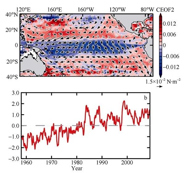
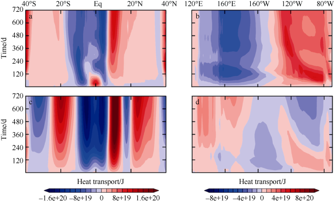
The spatial-temporal variability of heaving mode in the ocean is critical to understanding climate variability on interannual and decadal time scales. Using reanalysis data and a reduced gravity model, we investigated the leading heaving modes in the Pacific Ocean. The heaving signals are dominated by two modes: the first mode in which thermocline depth anomalies in the eastern and western equatorial Pacific have opposite signs, and the second mode in which thermocline depth anomalies in the equatorial and subtropical Pacific Ocean have opposite signs. The time evolution of these two heaving modes and the physics leading to these two modes were explored. Results indicate that the first mode is directly linked to equatorial zonal wind anomalies, and the second mode is induced by the wind stress curl anomaly in the subtropics. Furthermore, these two leading heaving modes have profound impacts on basin-scale heat transport (with an amplitude of 51014W) and ocean heat content redistribution (with an amplitude of 1.5×10²⁰J) through ocean waves and Ekman transport, highlighting the importance of heaving modes in modifying the variabilities of the climate system and climate change.
Key words: Heaving mode; Pacific Ocean; ocean wave; heat transport; climate change
Qihua Peng , Ruixin Huang , Weiqiang Wang , Dongxiao Wang . The main heaving modes in the Pacific Ocean[J]. Journal of Tropical Oceanography, 2020 , 39(2) : 1 -10 . DOI: 10.11978/2019038
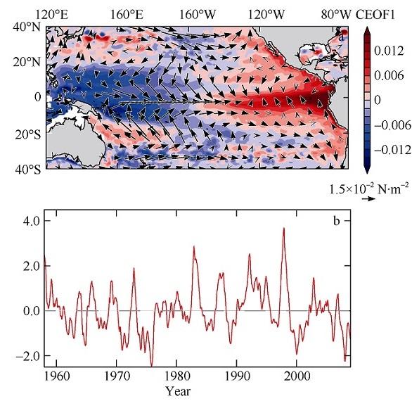
Fig. 1 CEOF1 (26%) of D15 anomalies (shading; dimensionless) and wind stress anomalies (vector; units: N·m-2) regressed against PC1 (a) and the corresponding PC time series (standardized) for CEOF1 (b) |
Tab. 1 Description of model experiments |
| Experiment | Forcing |
|---|---|
| EXP1 | Composite winds during the positive phase of CEOF1 |
| EXP2 | Composite winds during the negative phase of CEOF1 |
| EXP3 | Composite winds during the positive phase of CEOF2 |
| EXP4 | Composite winds during the negative phase of CEOF2 |
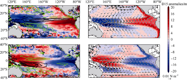
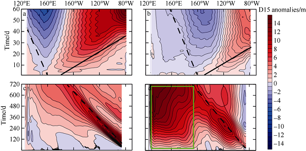
Fig. 3 Composite D15 anomalies (shading; units: m) of CEOF1 diagnosed from SODA (left panels) and from EXP1/EXP2 (right panels). Top panels are for the positive phase, and bottom panels, for the negative phase. Contours in the left panels indicate composite wind stress curl (contour interval=1×10⁻⁸ N·m-3, positive in black and negative in green), and vectors in the right panels denote composite wind stress anomalies (units: N·m-2). The output is obtained on day 120, a time for the Kelvin and Rossby waves to adjust to large D15 anomalies in the eastern and western equatorial Pacific Ocean |
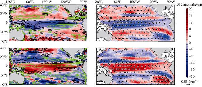
Fig. 4 Composite D15 anomalies (shading; units: m) of CEOF2 diagnosed from SODA (left panels) and from EXP3/EXP4 (right panels). Contours in the left panels indicate composite wind stress curl (contour interval=1×10⁻⁸ N·m-3, positive in black and negative in green), and vectors in the right panels denote composite wind stress anomalies (units: N·m-2). The output is obtained on day 360, a time for the Rossby waves and currents (much slower than Kelvin waves) to adjust to large D15 anomalies in the equatorial and subtropical Pacific Ocean |
Fig. 5 Hovmöller diagrams for simulated D15 anomalies (shading; units: m) from EXP1 along the equator (a) and the latitude band of 10°N (c). (b) and (d) are the same as (a) and (c), except for the outputs of EXP3. The solid black line indicates Kelvin wave propagation, and the dashed black line denotes Rossby wave propagation |
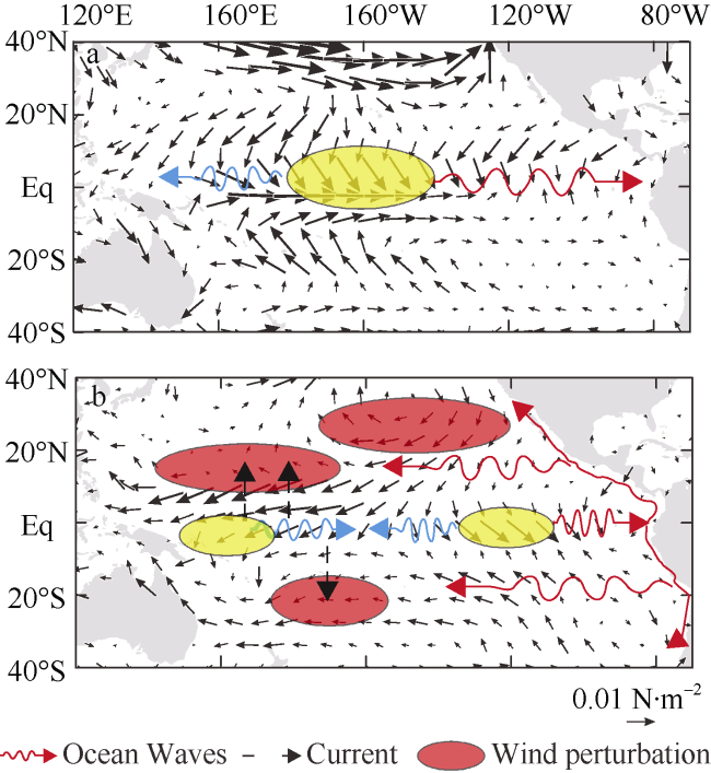
Fig. 6 Schematics for the first heaving mode (a) and the second heaving mode (b). Composite wind stress anomalies (vector; units: N·m-2) of the two modes are plotted. The wavy lines (downwelling in red and upwelling in blue) denote ocean waves (including Kelvin waves and Rossby waves), and the dashed vectors indicate wind-driven currents. The ellipses (downwelling-favorable wind anomalies in red and equatorial wind perturbations in yellow) indicate the key wind stress perturbation regions |
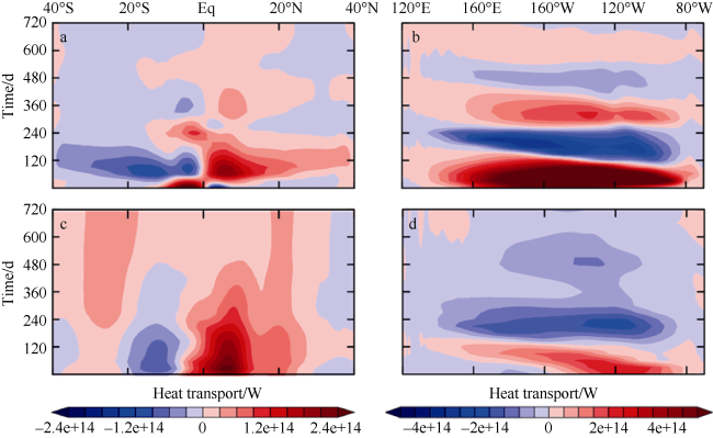
Fig. 7 Total heat transport (shading; units: W) of EXP1 in the meridional (a) and zonal directions (b). (c) and (d) are the same as (a) and (b), except for EXP3 |
| 1 |
|
| 2 |
|
| 3 |
|
| 4 |
|
| 5 |
|
| 6 |
|
| 7 |
|
| 8 |
|
| 9 |
|
| 10 |
|
| 11 |
|
| 12 |
|
| 13 |
|
| 14 |
|
| 15 |
|
| 16 |
|
| 17 |
|
| 18 |
|
| 19 |
|
| 20 |
|
| 21 |
|
| 22 |
|
| 23 |
|
| 24 |
|
| 25 |
|
| 26 |
|
| 27 |
|
| 28 |
|
| 29 |
|
| 30 |
|
| 31 |
|
| 32 |
|
| 33 |
|
| 34 |
|
| 35 |
|
| 36 |
|
| 37 |
|
| 38 |
|
| 39 |
|
| 40 |
|
| 41 |
|
/
| 〈 |
|
〉 |
