Biodiversity, biogeography and seasonal variation of zooplankton Collodarians (Radiolaria) in surface waters from the northern Indian Ocean to the South China Sea*

  • CHENG Xiawen , 1, 2 ,
  • ZHANG Lanlan , 2 ,
  • QIU Zhuoya 2, 3 ,
  • XIANG Rong 2 ,
  • CHANG Hu 2, 3
Expand
  • 1. State Key Laboratory of Marine Resources Utilization in South China Sea, College of Marine Science, Hainan University, Haikou 570228, China
  • 2. Key Laboratory of Ocean and Marginal Sea Geology, South China Sea Institute of Oceanology, Chinese Academy of Sciences, Guangzhou 511458, China
  • 3. University of Chinese Academy of Sciences, Beijing 100049, China
ZHANG Lanlan. email:

Copy editor: YIN Bo

Received date: 2022-03-11

  Revised date: 2022-04-24

  Online published: 2022-04-26

Supported by

National Natural Science Foundation of China(41876207)

National Natural Science Foundation of China(42176080)

Chinese Academy of Sciences Project(QYZDY-SSW-DQC005)

Chinese Academy of Sciences Project(Y4SL021001)

Abstract

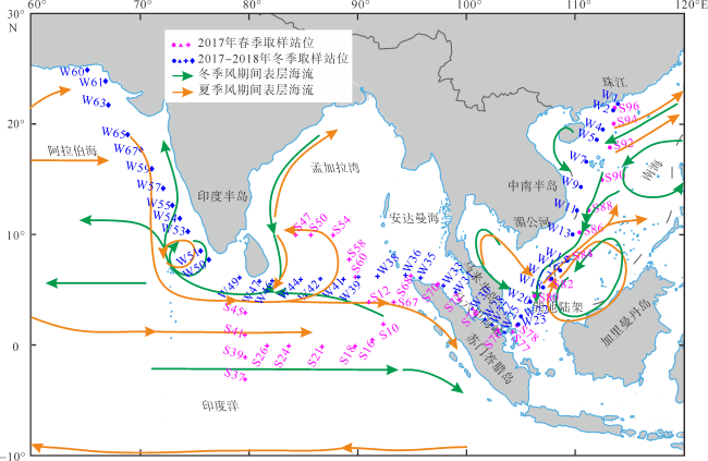
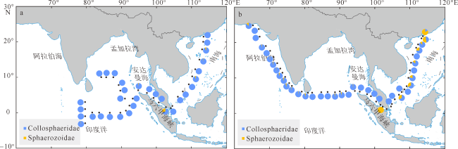
Zooplankton collodarians with symbiontes play important roles in the organic carbon cycle and silicon cycle in the oligotrophic waters. However, studies on the collodiarian geographic distribution were few. In this study, the biodiversity, biogeography and seasonal variation of collodarians in the surface water of the northern Indian Ocean (NIO), the Malacca Strait (MLS) and the South China Sea (SCS) are revealed for the first time by using the ship-board plankton net to collect samples and using the Rose Bengal stains to distinguish between “living” and “dead” specimens. Totally, the 17 species of collodarians occurred in spring, with 27 species in winter. The collodarian diversity in NIO and MLS is generally less than that in SCS in spring, while in the winter, the former is higher than the latter, indicating that the regional biodiversity from NIO to the SCS is considerably affected by the East Asian monsoon. Moreover, the changes of collodarian community structure have biogeographic differences under the influence of East Asian monsoon. For example, the family Collosphaeridae is obviously dominant both in spring and winter, while the family Sphaerozoidae is dominant only in winter; the composition of dominant species is also different between the spring and the winter, suggesting the collodairian community in surface water is significantly affected by the seasonal changes. Under the influence of East Asian monsoon, the mixing of surface water enhanced, resulting in obvious changes in the compostion of collodarian species, which indicates that seasonal changes are the main factor that controls the community structure of collodarians in the study sea area. The abundance of collodarians is closely related to the regional environment. For instance, the collodarian abundance is very low in spring and winter from MLS to the Sunda Shelf, followed by SCS, and is high in NIO, reflecting their adaptability to specific marine environment. It is assumed that the influence of habitat on a large scale is higher than the control of monsoon change. Therefore, the biodiversity and abundance of collodarians can reflect the different ecological environmental signals, which further provides important observation data and a basic reference for the reconstruction of palaeooceanography and palaeoenvironment by using the collodarian substitution indexes in the future.

Cite this article

CHENG Xiawen , ZHANG Lanlan , QIU Zhuoya , XIANG Rong , CHANG Hu . Biodiversity, biogeography and seasonal variation of zooplankton Collodarians (Radiolaria) in surface waters from the northern Indian Ocean to the South China Sea*[J]. Journal of Tropical Oceanography, 2023 , 42(2) : 97 -112 . DOI: 10.11978/2022047

作为海洋浮游原生动物放射虫(polycystine radiolaria)中唯一营群体生活的目阶类群(De Wever et al, 2001; Adl et al, 2019; 张杰 等, 2020), 胶体虫可能是寡营养海洋中最重要的浮游生物之一, 因为它的丰度高, 与细胞或群落内的大量共生体相关的初级生产力也很高, 从而影响了寡营养海洋中的有机碳固定(Ishitani et al, 2012; Biard et al, 2016; Zhang et al, 2018)。具有硅质骨骼的胶体虫也在海洋的硅循环中起着影响作用。胶体虫物种在地质历史上出现时间较晚, 是最年轻的放射虫生物地层标志种(Nigrini et al, 2001)。以往, 学者们主要关注胶体虫的分类学, 并将其分类地位从科阶提升至目阶单元(Haeckel, 1887; 陈木宏 等, 1996; 谭智源, 1998; 谭智源 等, 1999; De Wever et al, 2001; Suzuki et al, 2011; Biard et al, 2015; Adl et al, 2019; 张杰 等, 2020)。Biard等(2017)利用18S rDNA测序法分析了地中海胶体虫的科阶单元组成分布; Zhang等(2020)则从目阶单元角度指出南海胶体虫相较于罩笼虫和泡沫虫更偏喜相对稳定的水体环境。然而, 对胶体虫物种多样性与生物地理分布格局的研究较为薄弱。
北印度洋—南海位于低纬度海域, 是全球气候演变枢纽的重要组成部分, 跨越多个不同区域如南海、马六甲海峡、安达曼海和北印度洋等(图1)。本文依托2018年1月首次中国-巴基斯坦印度洋联合考察航次和2017年4月国家自然科学基金委东印度洋共享航次, 进行了北印度洋—南海走航断面表层水体样品的连续采集, 通过分析浮游生物胶体虫在不同区域下的物种多样性、揭示其生物地理分布特征和季节变化, 填补热带跨海域胶体虫多样性研究空白、提高生物多样性的认识, 为胶体虫在海洋生态系统中发挥的作用及其在古气候和古环境替代指标的研究等提供重要的观测数据和基础参考。
图1 北印度洋—南海断面春季和冬季表层水采样站位

表层水海流改自Zhang等(2020)和Schott等(2001)。该图基于国家测绘地理信息局标准地图服务网站下载的审图号为GS(2016)1663的标准地图制作, 底图无修改

Fig. 1 Spring and winter surface water sampling sites in the northern Indian Ocean-South China Sea section. Surface currents are modified from Zhang et al (2020) and Schott et al (2001)

1 材料和方法

研究材料是通过搭载国家自然科学基金委东印度洋春季综合科学考察共享航次(2017年3月10日至4月19日)和中国-巴基斯坦首次印度洋冬季联合考察航次(2017年12月31日至2018年2月5日)(航次编号: NORC2017-10), 利用走航水滤网装置(网孔直径为63μm)(Zhang et al, 2020), 连续走航采集表层水(水深约5m)的样品, 用5%甲醛溶液固定、冷藏保存, 留待实验室分析。春季南海至东印度洋断面37个样品, 跨越春季东印度洋、春季安达曼海、春季马六甲海峡、春季南海4个区域; 冬季南海至西北印度洋断面39个样品, 跨越冬季阿拉伯海、冬季东印度洋、冬季安达曼海、冬季马六甲海峡、冬季南海5个区域(图1, 表1)。走航表层水海表温度(SST)和海表盐度(SSS)数据均有同步获取(图2), 硅酸盐和磷酸盐数据来源于世界海洋图集(World Ocean Atlas, WOA) 2018, 基于1°×1°分辨率的1900—2017年的1月平均值和3月平均值, 分别对应冬季和春季的采样环境, 将原始数据插值到所有采样站位, 获得相应站位所在点的环境数据。
表1 走航水采集站位、经纬度、时间、样品流量以及胶体虫的物种数和总丰度

Tab. 1 Sites, latitude, longitude, the time of sampling, sampling flow, number of species and total abundance of collodarian (specimens per one-meter square)

站位 开始经度 开始纬度 结束经度 结束纬度 采样开始—结束时间 流量/L 种数/个 总丰度/
(个·m-3)
S10 92°34′35″E 1°59′58″N 92°03′06″E 3°00′02″N 2017/03/14 00:25—05:40 6379 4 34
S12 91°16′54″E 3°58′35″N 90°30′17″E 4°59′58″N 2017/03/15 04:15—09:25 5979 6 58
S16 91°34′36″E 0°33′31″N 91°00′11″E 0°00′09″N 2017/03/16 22:30—00:30 (03/17) 2991 3 5
S18 90°00′44″E 0°01′05″S 88°59′57″E 0°00′04″S 2017/03/17 17:25—21:41 3291 3 5
S21 87°00′40″E 0°02′26″S 86°00′05″E 0°00′04″N 2017/03/18 15:52—20:09 4626 4 15
S24 83°58′53″E 0°01′05″N 83°00′11″E 0°00′08″N 2017/03/19 23:26—03:30 (03/19) 6700 4 14
S26 82°00′44″E 0°02′27″N 81°59′29″E 0°59′58″S 2017/03/20 16:39—00:17 (03/21) 11242 6 18
S37 80°00′40″E 2°58′28″S 80°00′05″E 1°59′56″S 2017/03/24 17:02—22:25 12169 9 234
S39 80°00′06″E 1°00′26″S 79°54′59″E 0°01′02″S 2017/03/25 07:02—13:20 13029 6 23
S41 79°59′38″E 0°59′39″N 79°59′57″E 1°29′55″N 2017/03/26 16:22—18:45 3309 6 48
S45 80°01′06″E 3°00′28″N 79°00′13″E 2°30′09″N 2017/03/27 19:39—00:15 (03/28) 6986 7 106
S47 84°35′01″E 10°00′25″N 84°59′41″E 10°00′02″N 2017/04/05 02:00—05:00 4860 6 159
S50 85°59′14″E 10°00′5″N 86°29′57″E 10°00′03″N 2017/04/05 16:30—21:50 9600 6 39
S54 87°59′58″E 10°00′00″N 88°31′39″E 10°00′04″N 2017/04/07 04:06—07:05 5918 6 118
S58 89°30′04″E 7°48′26″N 89°43′55″E 7°02′44″N 2017/04/08 13:45—16:55 5919 6 45
S60 90°00′01″E 6°14′16″N 91°45′02″E 1°16′07″N 2017/04/09 23:04—18:50 (04/10) 36886 5 33
S67 93°31′21″E 3°58′03″N 94°57′12″E 6°13′24″N 2017/04/13 15:30—00:30 (04/14) 5207 5 54
S68 95°04′13″E 6°19′35″N 96°08′07″E 6°01′58″N 2017/04/14 02:00—06:00 3184 8 86
S70 97°32′28″E 5°34′59″N 98°04′03″E 5°23′52″N 2017/04/14 11:15—13:10 1500 3 72
S72 99°26′34″E 4°11′17″N 100°14′11″E 3°28′15″N 2017/04/14 19:36—23:50 3662 3 9
S74 100°55′16″E 2°52′51″N 101°42′30″E 2°20′29″N 2017/04/15 03:26—07:11 4216 3 2
S76 102°55′42″E 1°32′43″N 104°11′20″E 1°15′11″N 2017/04/15 12:16—17:50 5659 5 3
S77 104°20′27″E 1°17′36″N 104°43′38″E 1°51′45″N 2017/04/15 18:26—21:12 5955 2 2
S78 104°44′09″E 1°53′41″N 105°15′38″E 3°24′24″N 2017/04/15 21:20—03:31 (04/16) 5104 0 0
S80 106°19′34″E 4°31′18″N 107°17′53″E 5°31′38″N 2017/04/16 09:21—14:32 3817 5 2
S82 107°44′55″E 5°59′36″N 108°42′21″E 6°58′53″N 2017/04/16 20:22—01:29 (04/17) 5623 8 11
S84 109°26′04″E 8°00′14″N 109°52′57″E 9°01′21″N 2017/04/17 06:12—10:15 6873 6 11
S86 110°24′20″E 10°15′55″N 110°43′04″E 10°59′28″N 2017/04/17 14:59—17:51 5303 5 9
S88 111°15′36″E 12°15′26″N 111°42′58″E 13°19′07″N 2017/04/17 22:41—02:41 (04/18) 8553 6 29
S90 112°27′19″E 14°59′45″N 112°55′57″E 16°12′22″N 2017/04/18 09:03—13:45 2081 9 26
S92 113°12′14″E 17°54′41″N 113°25′45″E 19°13′06″N 2017/04/18 19:55—00:30 (04/19) 4578 11 65
S94 113°26′09″E 19°15′31″N 113°33′15″E 19°59′14″N 2017/04/19 06:02—09:12 3071 7 58
S96 113°36′49″E 21°29′10″N 113°36′49″E 21°29′10″N 2017/04/19 12:10—14:55 5536 6 11
W1 113°51′46″E 21°49′33″N 113°28′38″E 21°16′53″N 2017/12/31 13:21—15:48 6350 4 8
W2 113°27′02″E 21°14′30″N 112°31′57″E 20°29′54″N 2017/12/31 15:57—19:13 8467 5 6
W4 112°30′27″E 19°30′42″N 111°57′27″E 18°35′28″N 2017/12/31 23:16—03:10 (2018/01/01) 10109 9 27
W5 111°57′27″E 18°35′28″N 111°24′52″E 17°41′14″N 2018/01/01 03:17—06:57 9504 4 19
W7 110°59′39″E 16°36′21″N 110°44′00″E 15°31′08″N 2018/01/01 11:17—15:26 10757 2 16
W9 110°29′37″E 14°19′18″N 110°19′39″E 13°23′27″N 2018/01/01 19:43—23:01 8554 5 41
W11 110°08′02″E 12°12′26″N 109°55′06″E 11°02′54″N 2018/01/02 03:15—07:25 10800 9 17
W13 109°43′18″E 10°02′36″N 109°30′48″E 8°59′25″N 2018/01/02 11:03—14:49 9763 7 27
W15 109°13′46″E 7°41′43″N 108°37′56″E 6°49′44″N 2018/01/02 19:32—23:16 9677 3 16
W16 108°36′12″E 6°48′02″N 107°49′50″E 6°03′43″N 2018/01/02 23:24—03:15 (01/03) 9979 3 14
W17 107°49′10″E 6°03′06″N 107°01′02″E 5°15′49″N 2018/01/03 03:20—07:25 10584 1 2
W18 107°01′08″E 5°15′49″N 106°22′11″E 4°33′08″N 2018/01/03 07:25—11:05 9504 3 4
W20 105°50′16″E 3°59′14″N 105°18′10″E 3°25′44″N 2018/01/03 15:17—19:36 11189 1 0
W22 105°00′30″E 2°39′36″N 104°45′49″E 1°56′32″N 2018/01/03 23:30—03:25 (01/04) 10152 1 1
W23 104°44′30″E 1°55′37″N 103°58′42″E 1°14′59″N 2018/01/04 03:35—08:15 12096 0 0
W25 103°28′59″E 1°13′27″N 103°05′11″E 1°32′23″N 2018/01/04 10:10—12:08 5098 0 0
W27 102°22′27″E 1°53′19″N 101°45′10″E 2°22′26″N 2018/01/04 15:00—17:39 6869 1 1
W28 101°42′14″E 2°24′50″N 101°03′32″E 2°47′35″N 2018/01/04 17:52—20:47 7560 0 0
W30 100°31′45″E 3°20′55″N 99°00′15″E 4°51′22″N 2018/01/04 23:30—02:45 (01/05) 8424 1 6
W31 99°00′15″E 4°51′22″N 98°35′31″E 5°09′28″N 2018/01/05 07:49—11:15 8899 2 3
W33 97°53′43″E 5°26′39″N 96°59′05″E 5°45′41″N 2018/01/05 15:09—18:35 8813 1 6
W35 95°48′01″E 6°08′43″N 94°24′58″E 6°22′20″N 2018/01/05 23:10—04:10 (01/06) 12960 7 89
W36 94°24′20″E 6°22′05″N 93°10′42″E 6°20′14″N 2018/01/06 04:15—07:25 8208 8 187
W38 91°50′12″E 6°17′01″N 91°09′49″E 6°13′44″N 2018/01/06 12:05—15:33 8986 3 19
W39 90°05′46″E 6°13′38″N 89°53′13″E 6°12′08″N 2018/01/06 15:47—20:07 11232 7 53
W41 88°43′20″E 6°00′02″N 86°36′34″E 6°03′36″N 2018/01/07 00:30—07:00 16848 7 53
W42 86°36′34″E 6°03′36″N 85°24′59″E 6°00′39″N 2018/01/07 07:00—11:20 11232 8 47
W44 84°48′26″E 5°59′12″N 83°32′53″E 5°56′08″N 2018/01/07 14:40—19:18 12010 7 23
W46 82°11′45″E 5°52′11″N 81°01′51″E 5°49′35″N 2018/01/08 00:20—04:11 9979 9 47
W47 81°01′11″E 5°49′30″N 80°08′51″E 5°50′29″N 2018/01/08 04:20—07:25 7992 7 26
W49 79°12′20″E 6°10′02″N 76°23′57″E 7°46′30″N 2018/01/08 11:20—23:30 31536 11 64
W50 76°23′45″E 7°46′55″N 75°38′12″E 8°32′19″N 2018/01/08 23:40—03:35 (01/09) 10152 11 212
W51 75°37′44″E 8°33′10″N 75°00′04″E 9°22′07″N 2018/01/09 03:45—07:15 9072 10 109
W53 74°28′16″E 10°19′31″N 73°48′23″E 11°19′06″N 2018/01/09 11:30—15:56 11491 15 201
W54 73°42′28″E 11°29′44″N 73°03′41″E 12°38′17″N 2018/01/09 16:40—21:29 12485 12 317
W55 73°02′35″E 12°40′36″N 72°38′59″E 13°28′04″N 2018/01/09 21:39—00:59 (01/10) 8640 10 309
W57 72°12′13″E 14°11′45″N 71°43′50″E 14°59′05″N 2018/01/10 03:55—07:10 8424 16 120
W59 71°08′52″E 15°58′47″N 70°35′10″E 16°59′41″N 2018/01/10 11:20—15:42 11318 11 193
W60 65°14′32″E 24°54′00″N 65°15′03″E 24°50′35″N 2018/02/02 16:25—20:05 9504 5 13
W61 66°55′35″E 23°51′08″N 66°57′57″E 22°47′34″N 2018/02/04 21:20—01:20 (02/05) 10368 3 3
W63 67°11′19″E 21°42′47″N 68°04′34″E 20°32′54″N 2018/02/05 05:25—10:30 13176 6 9
W65 68°56′39″E 19°03′34″N 69°28′14″E 18°37′51″N 2018/02/05 16:04—19:40 9331 9 56
W67 70°10′07″E 17°41′06″N 70°42′41″E 16°45′22″N 2018/02/05 23:59—03:53 10109 6 66
图2 研究样品采集期间的水文环境

a. 冬季海表温度; b. 春季海表温度; c. 冬季海表盐度; d. 春季海表盐度; e. 冬季硅酸盐浓度; f. 春季硅酸盐浓度; g. 冬季磷酸盐浓度; h. 春季硅酸盐浓度。该图基于国家测绘地理信息局标准地图服务网站下载的审图号为GS(2016)1663的标准地图制作, 底图无修改

Fig. 2 Hydrological environment during the sampling periods. (a) sea surface temperature in winter; (b) sea surface temperature in spring; (c) sea surface salinity in winter; (d) sea surface salinity in spring; (e) silicate concentration in winter; (f) silicate concentration in spring; (g) phosphate concentration in winte; (h) phosphate concentration in spring

实验室内样品处理与制片方法与Zhang等(2020)相同, 首先选取全部或1/2样品用配置质量浓度为4%的虎红染色剂进行染色(区分出活体胶体虫), 染色时间约1 ~ 2h; 然后, 依次经过4个孔径(1mm、500μm、63μm和38.5μm)的筛网进行过筛, 用纯净水冲洗去掉浮色, 将其中较小孔径的3个筛网上的样本分别冲洗入烧杯内, 然后利用垂直沉降法进行浓缩收集入离心管内, 最后将样本均匀涂抹于载玻片上, 并用中性树胶和盖玻片进行封片、制成胶体虫(放射虫)玻片, 盖玻片规格为24mm×50mm (胡维芬 等, 2015; Zhang et al, 2020)。
胶体虫(放射虫)物种鉴定方法: 经镜检在0.5 ~ 1mm的薄片中未发现放射虫, 且考虑样品采集网孔径为63μm, 故本文样本物种鉴定的薄片为63 ~ 500μm。首先, 将研究样品出现的全部胶体虫个体进行不同形态的拍照, 根据其形态特征的相似或相近性进行归类, 然后依据前人研究资料(Haeckel, 1887; 陈木宏 等, 1996; 谭智源 等, 1999), 对不同形态的属种进行命名、作为活体放射虫鉴定图版。考虑到热带放射虫物种多样性较为丰富, 为了提高数据的可靠性和准确度, 丰度计算时每个样本统计> 1000个个体; 属种组成计算则每个样本鉴定统计> 500个个体, 如果样本薄片里的个体数量不足, 则全部鉴定统计。
统计分析方法: 利用Primer软件进行多样性的分析计算, 用简单分异度来表征物种数目, 香农-威尔指数指示胶体虫物种丰富度和均匀度, 用其来表征胶体虫的多样性(Shannon, 1948)。群落优势种根据优势度Y值来确定, 将Y > 0.02的物种定为优势种(沈国英 等, 2002)。依据胶体虫鉴定统计结果, 选取出现频率大于10%且相对丰度大于2%的15个胶体虫物种, 对北印度洋海域范围胶体虫分布区域进行Q型聚类分析, 聚类时去除了W60和W61站位, 以避免陆架浅水区胶体虫丰度和物种多样性过低对聚类结果产生干扰。聚类利用数理统计软件SPSS23欧式距离的方法。

2 结果

2.1 样品采集期间的水文环境

研究海域的春季温度明显高于冬季, 盐度春季略高于冬季。关于温度的变化, 春季东北印度洋至马六甲海峡的温度最高介于29.46 ~ 31.26℃, 南海断面的温度由北边靠近珠江口较低向南部增高, 变化幅度较大(24.95 ~ 30.14℃)。冬季北印度洋除了最西北边较低之外至马六甲海峡的温度相对较高(26.58 ~ 29.30℃), 冬季南海断面的温度相对较低, 除北边靠近珠江口低于21.41℃外, 变化幅度介于25.13 ~ 27.93℃(图2b)。关于盐度的变化, 春季和冬季马六甲海峡—安达曼海的海表盐度均低于32.08‰; 南海的海表盐度春季除最北边珠江口(24.95‰)变化幅度为31.64‰ ~ 33.57‰, 冬季盐度介于29.28‰ ~ 32.95‰; 东北印度洋即孟加拉湾南部断面盐度的季节变化不明显、相对较低(< 33.18‰); 东北印度洋赤道断面春季海表盐度和西北印度洋冬季海表盐度均呈现高值, 最高达到35.43‰ (图2c, 2d)。

2.2 胶体虫物种多样性与丰度

北印度洋—南海表层水体中胶体虫在春季的物种数有17个, 冬季的物种数有27个, 两个季节共有的种类有16个。其中马六甲海峡出现的物种数最低(< 5个), 冬季北印度洋较高, 尤其是印度半岛西南部海域(> 10个)(图3a, 3b)。胶体虫群落的多样性呈现出区域差异和季节变化。春季, 印度洋至马六甲海峡胶体虫的多样性低于南海的多样性, 前者0.53 ~ 1.55, 后者为1.28 ~ 1.80; 冬季, 印度洋胶体虫的多样性显著增高(0.69 ~ 2.08), 南海次之(0 ~ 2.08), 马六甲海峡最低(0 ~ 0.27)(图3c, 3d)。
图3 胶体虫在冬季和春季的物种数和多样性变化

a. 冬季物种数; b. 春季物种数; c. 冬季多样性; d. 春季多样性。该图基于国家测绘地理信息局标准地图服务网站下载的审图号为GS(2016)1663的标准地图制作, 底图无修改

Fig. 3 Variation in species number and diversity of collodarians in winter and spring. (a) species number in winter; (b) species number in spring; (c) diversity in winter; (d) diversity in spring
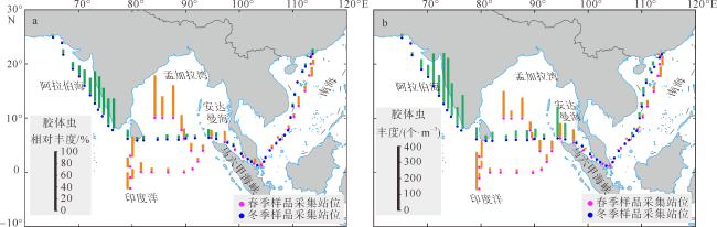
胶体虫的相对丰度即其在多囊虫类放射虫中的占比在春季和冬季的变化, 如图4a所示, 春季, 东印度洋胶体虫的相对丰度(1% ~ 68%)高于南海(0 ~ 16%)和马六甲海峡区域(1% ~ 7%); 冬季, 印度半岛西南端有一个异常高值区(43% ~ 54%)。南海至东印度洋, 冬季的胶体虫相对丰度(0 ~ 13%)明显低于春季(0 ~ 68%)。
图4 北印度洋—南海春季和冬季胶体虫的相对丰度(a)和丰度(b)变化

马六甲海峡部分站位无胶体虫。该图基于国家测绘地理信息局标准地图服务网站下载的审图号为GS(2016)1663的标准地图制作, 底图无修改

Fig. 4 Relative abundance (a) and absolute abundance (b) of Collodaria in spring and winter in the northern Indian Ocean-South China Sea. There is no collodarian observed at sites W23, W25 and W28 in the MLS
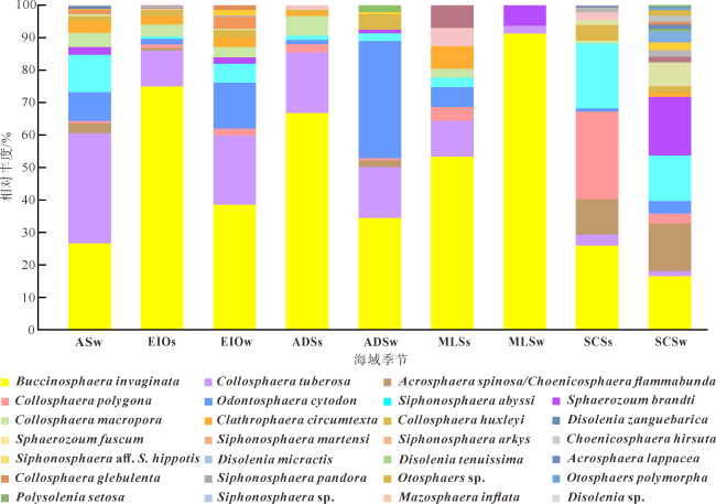
胶体虫的绝对丰度的季节变化如图4b所示, 春季, 东印度洋胶体虫的丰度(5 ~ 234个·m-3)总体上高于南海(0 ~ 65个·m-3)和马六甲海峡区域(2 ~ 9个·m-3); 冬季, 除了马六甲海峡至南海南部的巽他陆架较低之外, 其他海域相对较高, 尤其是在印度半岛西南端异常增高(109 ~ 317个·m-3)。在南海开放性海域和安达曼海乃至东印度洋断面, 胶体虫的丰度冬季(0 ~ 187个·m-3)明显高于春季(0 ~ 86个·m-3)。

2.3 胶体虫的属种组成与优势种变化

共发现胶体虫两个科Collosphaeridae和Sphaerozoidae, 未发现Collophidiidae科, 而且Collosphaeridae和Sphaerozoidae在不同海域和不同季节下的组成变化也不同, 如图5所示。春季, Collosphaeridae占据绝对优势, 尤其是在东印度洋海域, 高达99% ~ 100%; 冬季, Sphaerozoidae的占比虽出现增加, 但除极个别站点外(W1、W2、W25), 大部分海域的主导优势科依旧是Collosphaeridae (> 88%)。
图5 春季(a)和冬季(b)不同海域胶体虫的群落结构(科阶)变化

马六甲海峡部分站位(W23、W25、W28)无胶体虫。该图基于国家测绘地理信息局标准地图服务网站下载的审图号为GS(2016)1663的标准地图制作, 底图无修改

Fig. 5 Variation of community structure at the collodarian family level in spring (a) and winter (b). There is no collodarian at sites (W23, W25 and W28) in the MLS

胶体虫的属种组成季节变化也呈现出区域性的差异, 如图6所示。南海春季 Buccinosphaera invaginataCollosphaera polygonaSiphonosphaera abyssi 3个物种的占比达70%以上。南海冬季的优势种不明显, B. invaginataS. abyssiAcrosphaera spinosa / Choenicosphaera flammabundaSphaerozoum brandti的相对丰度均为14% ~ 18%; 马六甲海峡春季和马六甲海峡冬季 B. invaginata的相对丰度大于50%, 且该种冬季占比显著高于春季; B. invaginata在东印度洋和安达曼海则相反, 春季显著高于冬季; 东印度洋春季和安达曼海春季的属种组成相近, 主要以B. invaginata为主导(> 67%); 安达曼海冬季和东印度洋冬季乃至阿拉伯海冬季的属种组成较为相近, B. invaginataC. tuberosaO. cyrtodon 3个物种的占比较高。值得注意的是, Sphaerozoum brandti只在冬季出现。
图6 不同海域春季和冬季胶体虫的物种组成变化

ASw: 阿拉伯海冬季; EIOs: 东印度洋春季; EIOw: 东印度洋冬季; ADSs: 安达曼海春季; ADSw: 安达曼海冬季; MLSs; 马六甲海峡春季; MLSw: 马六甲海峡冬季; SCSs: 南海春季; SCSw: 南海冬季

Fig. 6 Composition of collodarian species in spring and winter in each sea areas. ASw: Arabian Sea in winter; EIOs: eastern Indian Ocean in spring; EIOw: eastern Indian Ocean in winter; ADSs: Andaman Sea in spring; ADSw: Andaman Sea in winter; MLSs: Malacca Strait in spring; MLSw: Malacca Strait in winter; SCSs: south China sea in spring; SCSw: south China sea in winter

基于优势度划分出来的优势种如表2所示, 春季和冬季共同出现的优势种有两个即B. invaginataC. tuberosa, 前者在春季优势度指数(Y = 0.6214)显著高于冬季(Y = 0.2210)、后者则在冬季的优势度指数(Y = 0.1523)高于春季(Y = 0.0904), B. invaginataC. tuberosa均主要分布于北印度洋(分别为1 ~ 195个·m-3和0 ~ 117个·m-3), 在南海(分别为0 ~ 21个·m-3和0 ~ 4个·m-3)、马六甲海峡(分别为0 ~ 7个·m-3和0 ~ 1个·m-3)丰度较低(图7)。春季特有的优势种是C. polygona (Y = 0.0296), 主要分布在南海北部(0 ~ 26个·m-3)(图7)。冬季才出现的优势种有2个即O. cyrtodon (Y = 0.0660)和S. abyssi (Y = 0.0480), O. cyrtodon主要分布在北印度洋(0 ~ 70个·m-3), 在南海(0 ~ 5个·m-3)和马六甲海峡(0 ~ 1个·m-3) 分布较少, 而S. abyssi在阿拉伯海区域丰度较高(0 ~ 69个·m-3), 其次为南海(0 ~ 17个·m-3), 在东印度洋丰度较小(0 ~ 7个·m-3)(图7)。
表2 研究区胶体虫物种在春季和冬季表层水体中的优势度(Y)

Tab. 2 Dominance degree of collodarian species in spring and winter surface water in the studied areas

胶体虫种名 春季优势度 冬季优势度
Acrosphaera lappacea (Haeckel) 0.0001 0.0009
Acrosphaera spinosa (Haeckel) / Choenicosphaera flammabunda Haeckel 0.0069 0.0104
Buccinosphaera invaginata Haeckel 0.6214 0.2210
Choenicosphaera hirsuta (Ehrenberg) 0.0010 0.0002
Clathrophaera circumtexta Haeckel 0.0054 0.0075
Collosphaera glebulenta Bjørklund & Goll 0.0000 0.0002
Collosphaera huxleyi Müller 0.0092 0.0075
Collosphaera macropora Popofsky 0.0192 0.0116
Collosphaera polygona Haeckel 0.0296 0.0027
Collosphaera tuberosa Haeckel 0.0904 0.1523
Disolenia micractis (Ehrenberg) 0 0.0001
Disolenia sp. 0 0.0000
Disolenia tenuissima (Hilmers) 0 0.0002
Disolenia zanguebarica Ehrenberg 0.0005 0.0023
Mazosphaera inflata (Haeckel) 0 0.0000
Odontosphaera cyrtodon Haeckel 0.0058 0.0660
Otosphaera polymorpha Haeckel 0 0.0000
Otosphaers sp. 0 0.0000
Polysolenia setosa Ehrenberg 0 0.0000
Siphonosphaera abyssi (Ehrenberg) 0.0188 0.0480
Siphonosphaera aff. S. hippotis (Haeckel) 0 0.0015
Siphonosphaera arkys Su 0 0.0032
Siphonosphaera martensi Brandt 0.0001 0.0001
Siphonosphaera pandora (Haeckel) 0.0000 0.0001
Siphonosphaera sp. 0 0.0000
Sphaerozoum brandti Popofsky 0 0.0183
Sphaerozoum fuscum Meyen 0.0015 0

注: 加粗表示Y > 0.02

图7 胶体虫优势种在春、冬季的绝对丰度和相对丰度分布

a1 ~ a4: Buccinosphaera invaginata; b1 ~ b4: Collosphaera tuberosa; c1 ~ c4: Odontosphaera cyrtodon; d1 ~ d4: Siphonosphaera abyssi; e1 ~ e4: Collosphaera polygona。该图基于国家测绘地理信息局标准地图服务网站下载的审图号为GS(2016)1663的标准地图制作, 底图无修改

Fig. 7 Absolute and relative abundances of dominant collodarian species in spring and winter, a1~a4: Buccinosphaera invaginata; b1~b4: Collosphaera tuberosa; c1~c4: Odontosphaera cyrtodon; d1~d4: Siphonosphaera abyssi; e1~e4: Collosphaera polygona
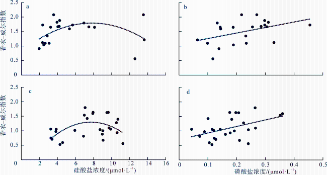
2.4 聚类分析结果

Q型聚类结果如图8所示, 分为类型Ⅰ和类型Ⅱ, 较好地代表了其季节特征。除了S16、S18、W67 3个异常点, 类型Ⅰ为春季站位, 类型Ⅱ为冬季站位。类型Ⅰ的胶体虫类群主要由B. invaginataC. tuberosa组成(76% ~ 94%), 类型Ⅱ的胶体虫类群主要由B. invaginataC. tuberosaO. cyrtodonS. abyssi组成(63% ~ 100%)。
图8 北印度洋春冬季胶体虫数据的Q型聚类分析结果

a. 聚类分析树状图; b. 聚类结果在站位图中的分布情况, 粉色代表类型Ⅰ, 蓝色代表类型Ⅱ。图a中的红色虚线表示。该图基于国家测绘地理信息局标准地图服务网站下载的审图号为GS(2016)1663的标准地图制作, 底图无修改

Fig. 8 Q-type cluster analyses of Collodaria data in spring and winter in the North Indian Ocean

3 讨论

3.1 不同海域的胶体虫丰度、多样性及其环境适应性

基于不同区域的环境差异, 划分出3个海域进行分析讨论: 南海属于半封闭性边缘海(王雪松 等, 2022); 马六甲海峡属于相对较为封闭的近海海域, 与外界水交换较弱(Zhang et al, 2020); 北印度洋属于开放性大洋。
Zhang等(2020)对南海至马六甲海峡的多囊虫类放射虫进行研究时, 已对南海海域进行Q型聚类分析, 将放射虫分为与冬季、春季和大陆架浅水区的混合信号有关的3种区系, 并将胶体虫的相对丰度即其在多囊虫类放射虫中的占比进行了较为详细的探讨, 指出胶体虫能够利用光合藻类共生体提供的营养物质生存, 贫营养对胶体虫的不利影响小于其对泡沫虫和罩笼虫的抑制作用, 而且胶体虫对南海春季稳定的贫营养水体环境的适应性较强, 相对丰度较高, 但其对于胶体虫的丰度和物种多样性的分析是欠缺的。南海胶体虫的丰度出现同一季节海盆区高、陆架区低的格局, 表明在南海胶体虫的丰度和与水深关系密切(图4)。相较于丰度, 南海的胶体虫多样性分布在陆架区和海盆区变化幅度不大、几乎看不出明显的界线。这与胶体虫在地中海的多样性变化不同, 前人研究发现地中海胶体虫的多样性会随着大洋条件的增强而增加, 其中大洋条件的程度主要是通过离岸距离和水深进行判定(Biard et al, 2017), 这可能与南海属于半封闭性边缘海的地理位置有关。
作为开放性大洋的北印度洋环境影响因素更为多元化, 北印度洋北部被亚欧大陆阻隔, 东邻巽他大陆架, 印度半岛分隔整个北印度洋为孟加拉湾和阿拉伯海, 由于靠近亚欧大陆, 印度洋海气相互作用强烈(Schott et al, 2001; 刘颖 等, 2020)。在春季, 孟加拉湾通过降水和河流径流接收大量淡水, 使海表盐度降低, 并保持强烈的盐度分层, 形成较厚的屏障层(Girishkumar et al, 2011), 相对稳定的水体有利于该区域胶体虫的繁盛, 因而孟加拉湾出现较高的胶体虫丰度。在赤道印度洋, 春季存在强烈向东流的赤道印度洋洋流(Wyrtki急流), 将阿拉伯海的高盐水向东输送, 导致东印度洋的上层海水混合增强(Wyrtki, 1973; Zeng et al, 2012), 在赤道区域的胶体虫相应表现出较低的丰度。值得注意的是, 冬季印度半岛西南岸外的海域具有非常高的胶体虫丰度(图3图4)。东北季风在阿拉伯海北部引起强烈的对流混合, 使得阿拉伯海西北部的混合层深度加深(Shankar et al, 2016), 但在阿拉伯海东南部, 西印度沿岸流将来自孟加拉湾的淡水向西输送, 造成阿拉伯海西南部低盐度和密度分层, 从而限制混合层深度并形成厚屏障层, 抑制了营养物质进入上层水体, 形成温暖、贫营养的水体条件(Masson et al, 2005; Gupta et al, 2016; Vijith et al, 2016)。胶体虫大多具有光合共生藻(甲藻)(Biard et al, 2017), 甲藻因其具有游泳能力和浮力被认为在低湍流的稳定水柱中也能积极获取营养(Xiang et al, 2019)。可见, 水体稳定性是影响北印度洋胶体虫丰度变化的主要因素。
胶体虫与多囊虫类放射虫的其他目阶单元不同, 缺乏骨针等结构、硅化程度较低, 对海水的硅酸盐高浓度的依赖性较低, 但Biard等(2017)指出硅酸盐浓度的增加可能会引起胶体虫形态上的多样性, 呈线性相关。本研究发现硅酸盐对胶体虫的多样性具有一定的促进作用, 但当硅酸盐浓度达到一定水平(~8μmol·L-1)时, 其对胶体虫多样性的促进作用就不再明显(图9a, 9c)。而磷酸盐浓度与胶体虫的多样性则在南海、北印度洋海域表现出正相关(图9b, 9d), 这可能与胶体虫的共生甲藻有关, 磷是藻类生长必不可少的营养元素, 尤其在寡营养海域(黄锦平 等, 2022)。与开放性大洋相比, 春季南海和东印度洋的硅酸盐和磷酸盐浓度均较高(图2), 因此南海到东印度洋的种数也较为一致, 春季南海的胶体虫多样性高于东印度洋, 表明南海胶体虫的均匀度较高。而在冬季, 阿拉伯海东南部磷酸盐的多样性高于南海的大部分站位, 北印度洋的胶体虫多样性高于南海。
图9 南海、北印度洋胶体虫多样性与采样站环境变量之间的相关性

a. 冬季胶体虫多样性与硅酸盐浓度的关系; b. 春季胶体虫多样性与硅酸盐浓度的关系; c. 冬季胶体虫多样性与磷酸盐浓度的关系; d. 春季胶体虫浓度与磷酸盐浓度的关系。图中黑色圆点为实际数据, 虚线为拟合线

Fig. 9 Correlations between the collodarian diversity and mean environment variables across the sampling sites. (a) relation with the silicate concentration in winter; (b) relation with the silicate concentration in spring; (c) relation with the phosphate concentration in winter; (d) relation with the phosphate concentration in spring

因此, 胶体虫的丰度与多样性的海洋环境影响因素是不一样的, 丰度与水深、水体稳定性相关, 多样性受控于硅酸盐和磷酸盐浓度。也就是说, 胶体虫丰度和多样性的高低能够反映出不同的海洋环境变化, 这对今后利用胶体虫相关指标进行古海洋环境研究具有很好的应用价值。
由于数据库分辨率的原因, 南海、北印度洋近岸的部分站位, 以及马六甲海峡站位的硅酸盐和磷酸盐数据部分缺失。马六甲海峡的胶体虫多样性在春、冬两季都处在较低的水平, 这可能与马六甲海峡所处地理位置有关。马六甲海峡呈东南—西北走向(图1), 形状为一狭长的喇叭形, 最宽处为200海里, 水深范围一般为30~130m, 与外界水体交换较弱(俞慕耕, 1987; 范锦晓 等, 2020; Zhang et al, 2020)。如图2所示, 在降雨和地表径流的强烈影响下, 马六甲海峡海水盐度相对较低, 这可能是导致马六甲海峡胶体虫物种多样性低的最主要因素。马六甲海峡春季多样性高于冬季, 海水盐度春季高于冬季(图2)。有研究表明马六甲海峡春季的硅酸盐含量较冬季会有所增加(Li et al, 2013), 春季较高的硅酸盐水平能会导致马六甲海峡春季相对较高的胶体虫多样性。马六甲海峡除会受到陆源影响外, 作为重要的海运枢纽, 世界贸易的快速发展加重了海峡污染, 季节和区域尺度上也发现营养盐浓度具有高度可变性, 这些环境变化会影响物种结构和初级生产力, 同时海峡的表层水体还极易受到扰动(Li et al, 2013; 王磊 等, 2015)。Zhang等(2020)的研究中多囊虫类放射虫的低胶体虫含量和的高罩笼虫含量也体现在马六甲海峡, 前者喜好水体层化强的水体环境、后者对高营养盐浓度响应敏感。可见, 受陆地环境影响显著的马六甲海峡胶体虫多样性和丰度均较低、但具有明显的季节变化, 推测受季风降雨影响下大量淡水输入导致的低盐、以及表层水体的强混合是控制胶体虫在马六甲海峡物种低多样性和低绝对丰度的关键因素。

3.2 胶体虫典型组合对季节变化的响应

北印度洋—马六甲海峡—南海断面表层水体中, 春季和冬季只发现了胶体虫的两个科Collosphaeridae和Sphaerozoidae, 未发现Collophidiidae科, 后者被认为生活在相对更深的水层中(Biard et al, 2017)。Collosphaeridae和Sphaerozoidae这两个科分布存在地理差异, Sphaerozoidae科在近海生物群落中的贡献较高, 而Collosphaeridae主要在远洋生物群中占据主要地位(Biard et al, 2017)。本文研究发现, Collosphaeridae科是热带北印度洋至南海胶体虫的优势科阶类群, 但Sphaerozoidae科的占比在半封闭性边缘海南海和马六甲海峡等的相对丰度比在北印度洋海域显著提升。且Collosphaeridae科和Sphaerozoidae科呈现出显著的季节变化, 春季Collosphaeridae科占据绝对优势, 尤其是在东印度洋海域, 高达99% ~ 100%; Sphaerozoidae的占比主要是在冬季出现明显波动, 尤其是在南海和马六甲海峡区域(图5)。
Collosphaeridae科一般具有球形的硅质壳体, 归属于这个科的很多胶体虫属种都具有光合共生藻(Biard et al, 2017)。这种含光合共生藻的胶体虫是在赤道太平洋现今海洋环流系统和贫营养条件形成之后进化而来的, 以便适应逐渐变得贫营养的热带海域(Ishitani et al, 2012)。这些共生藻不但为胶体虫提供了生存所需营养, 也为亚热带和热带的贫营养海域提供高的初级生产力(Ishitani et al, 2012)。尽管春季热带、亚热带海洋的养分供应减少, Collosphaeridae科胶体虫仍然可以靠体内的光合内共生体提供营养, 从而成为胶体虫目中的优势类群。Sphaerozoidae科则主要由硅化程度低、结构较为松散的骨针构成。南海和马六甲海峡在冬季受东北季风影响下, 强烈的垂直混合将大量的营养物质从下层水体带至表层水体(俞慕耕, 1987; Zhang et al, 2020)。值得注意的是, Sphaerozoidae科相对丰度变化具有明显的季节波动, 尤其是在个别站位冬季明显增加、甚至超过Collosphaeridae科, 表明Sphaerozoidae科的生物学和生态特征显著不同于Collosphaeridae科, 值得以后进一步探究, 尽管它们在海底沉积物中因保存问题、很难作为古海洋和古气候研究的替代指标。
基于Q型聚类分析结果, 北印度洋海域胶体虫按季节分为类型Ⅰ和类型Ⅱ, 分别对应春季与冬季两个季节区系。类型Ⅰ主要由B. invaginataC. tuberosa组成, 类型Ⅱ主要由B. invaginataC. tuberosaO. cyrtodonS. abyssi组成, 表明两个类型胶体虫的属种组成也具有显著的季节差异。此外, 除了马六甲海峡, 胶体虫主要属种组成在冬季比在春季更具多样性(图6)。目前为止, 对于胶体虫属种的生物学和生态特征研究较为薄弱, 一定程度上限制了本项研究对胶体虫属种的深入讨论。在北印度洋—安达曼海—马六甲海峡—南海, 在春季和冬季均具有高优势度的B. invaginata也呈现出季节变化: 除了在马六甲海峡B. invaginata的冬季优势高于春季, 其他区域则是B. invaginata冬季优势低于春季(图6图7), 推测与马六甲海峡特有的地理区域环境, 以及冬季更为多样化的属种组成密切相关。B. invaginata在春季东印度洋的相对丰度最高, 认为与海水表面高温有一定相关性。Boltovskoy等(2010)发现B. invaginata主要分布在热带低纬度地区。研究发现较高的温度通常会增加参与光合作用过程的酶的活性, 从而促进光合制氧和碳固定, 进而导致与B. invaginata共生的浮游植物(甲藻)的生长(Bissinger et al, 2008; Biard et al, 2017)。基于本文观测数据结果, 我们推测B. invaginata可能对高温(> 29℃)具有较强的耐受性和适应性。但是值得注意的是, 过高的温度可能会导致浮游植物的光合机能受损, 降低光合能力(Mai et al, 2021)。因此, B. invaginata耐高温的上限尚未知。
B. invaginata一样, 作为放射虫生物地层最年轻的地层种(Nigrini et al, 2001), C. tuberosa也是亚热带和热带浅水种, 在西太平洋暖池具有较高的丰度, 一直被视为贫营养和稳定水层的指示种(Yamashita et al, 2002)。C. tuberosa在北印度洋相对丰度冬季高于春季, 但在南海和马六甲海峡则是春季高于冬季(图6图7), 表明该种具有较为宽广的温度适应性(26.58 ~ 29.3℃), 且其季节变化受地理格局影响。此外, 胶体虫物种O. cyrtodon的生态分布研究报道较少, 前人多关注其分类学上的形态特征描述(Haeckel, 1887; 斯特列尔科夫 等, 1962; De Wever et al, 1990)。O. cyrtodon丰度和相对丰度均呈现出北印度洋冬季高于春季、南海和马六甲海峡冬春季变化幅度小的特征(图7), 表明O. cyrtodon对季节变化的响应程度也体现出地理格局上的差异。有报道发现S. abyssi在西北太平洋生活在200 ~ 500m的次表层-中上部水体中, 受温度约为 16 ~ 18℃北太平洋副热带模态水的影响(Matsuzaki et al, 2020)。在本研究中, S. abyssi在春季和冬季的南海, 和冬季的阿拉伯海均有出现, 这些海域的温度均在25℃以上, 从而拓展了对S. abyssi生活水温的认知。

4 结论

本文通过大量观测样品和系统的研究, 对北印度洋—南海跨越多个海域的浮游动物胶体虫的物种多样性、生物地理和季节变化提供了一些新的认识。
1) 北印度洋—南海胶体虫物种较为丰富, 春季有17种、冬季有27种, 主要以Collosphaeridae科和Sphaerozoidae科为主, 未发现Collophidiidae科; 春、冬季共同出现的优势种有B. invaginataC. tuberosa, 后者在冬季的优势较春季强; C. polygona是春季特有的优势种, O. cyrtodonS. abyssi是冬季特有的优势种, 表明研究区表层水体中胶体虫的群落结构受东亚季风影响显著, 季节变化是控制群落结构的主因。
2) 胶体虫生物多样性的地理分布受东亚季风显著影响, 在春季北印度洋—马六甲海峡的多样性普遍低于南海, 但在冬季北印度洋的多样性则高于南海。马六甲海峡胶体虫多样性在春、冬季皆为最低水平, 这可能与海峡地区较低的盐度和较强的水体混合有关; 南海、北印度洋胶体虫多样性与营养盐的季节变化有关, 丰富的硅酸盐和磷酸盐则有利于促进胶体虫多样性的提高。
3) 胶体虫的丰度与区域环境密切相关, 如马六甲海峡至巽他陆架春、冬季均较低, 南海次之, 北印度洋春、冬季都相对较高, 反映出其对特定海洋环境的适应性, 推测大尺度下区域的影响要高于季风变化的控制, 胶体虫丰度在南海、马六甲海峡等边缘海/近岸区域与水深和盐度密切相关, 而在开阔大洋北印度洋则主要与水体稳定性相关。
胶体虫的物种多样性和绝对丰度能够反映出不同的生态环境信号, 可作为古海洋和古环境重建研究的替代指标。
[1]
陈木宏, 谭智源, 1996. 南海中、北部沉积物中的放射虫[M]. 北京: 科学出版社:1-271.

CHEN MUHONG, TAN ZHIYUAN, 1996. Radiolaria from surface sediments of the central and northern South China Sea[M]. Beijing: Science Press: 1-271. (in Chinese with English abstract)

[2]
范锦晓, 胡松, 2020. 潮汐和风对马六甲海峡海流的影响[J]. 热带海洋学报, 39(4): 13-24.

DOI

FAN JINXIAO, HU SONG, 2020. Impact of tides and winds on currents in the Malacca Strait[J]. Journal of Tropical Oceanography, 39(4): 13-24. (in Chinese with English abstract)

DOI

[3]
胡维芬, 张兰兰, 陈木宏, 等, 2015. 南海断面春季活体放射虫生态分布及其对环境的响应[J]. 中国科学: 地球科学, 45(1): 83-98.

HU WEIFEN, ZHANG LANLAN, CHEN MUHONG, et al, 2015. Distribution of living radiolarians in spring in the South China Sea and its responses to environmental factors[J]. Science China: Earth Sciences, 45(1): 83-98. (in Chinese with English abstract)

[4]
黄锦平, 吴泽涛, 苏玉萍, 等, 2022. 不同浓度和形态磷模拟调控浮游植物群落演替实验[J]. 环境科学学报, 42(2): 422-429.

HUAGN JINPING, WU ZETAO, SU YUPING, et al, 2022. Experiments on simulation regulation of phytoplankton community succession with different concentrations and forms of phosphorus[J]. Acta Scientiae Circumstantiae, 42(2): 422-429. (in Chinese with English abstract)

[5]
刘颖, 严幼芳, 凌征, 2020. 北印度洋障碍层厚度气候态和季节变化特征及其成因初步分析[J]. 热带海洋学报, 39(5): 98-108.

DOI

LIU YING, YAN YOUFANG, LING ZHENG, 2020. Preliminary analysis on climatological and seasonal variation of barrier layer thickness in the northern Indian Ocean and it’s mechanism[J]. Journal of Tropical Oceanography, 39(5): 98-108. (in Chinese with English abstract)

DOI

[6]
沈国英, 施并章, 2002. 海洋生态学[M]. 北京: 海洋生态学:158-159.

SHEN GUOYING, SHI BINGZHANG, 2002. Marine Ecology[M]. Beijing: Marine Ecology: 158-159. (in Chinese with English abstract)

[7]
斯特列尔科夫 A A, 列雪特妮阿克 V V, 1962. 中国南海海南岛南端地区的群体放射虫[J]. 海洋科学集刊, 1: 121-139.

Strelkov A A, Reshetnjak V V, 1962. Kolonialnye radiolyarii Spumellaria mirovogo okeana[J]. Studia Marine Sinica, 1: 121-139. (in Chinese with English abstract)

[8]
谭智源, 1998. 中国动物志[M]. 北京: 科学出版社:1-360.

TAN ZHIYUAN, 1998. Fauna of China[M]. Beijing: Science Press: 1-360. (in Chinese with English abstract)

[9]
谭智源, 陈木宏, 1999. 中国近海的放射虫[M]. 北京: 科学出版社:1-404.

TAN ZHIYUAN, CHEN MUHONG, 1999. Radiolaria off the coast of China[M]. Beijing: Science Press: 1-404. (in Chinese with English abstract)

[10]
王磊, 冷晓云, 孙庆杨, 等, 2015. 春季季风间期巽他陆架和马六甲海峡表层海水浮游植物群落结构研究[J]. 海洋学报, 37(2): 120-129.

WANG LEI, LENG XIAOYUN, SUN QINGYANG, et al, 2015. The distribution of phytoplankton community structure in the Sunda Shelf and the Strait of Malacca during spring intermonsoon[J]. Haiyang Xuebao, 37(2): 120-129. (in Chinese with English abstract)

[11]
王雪松, 陈忠, 许安涛, 等, 2022. 南海东北部深海盆末次冰盛期以来陆源碎屑粒度特征及影响因素[J]. 热带海洋学报, 41(1): 158-170.

DOI

WANG XUESONG, CHEN ZHONG, XU ANTAO, et al, 2022. Grain size characteristics and influencing factors of terrigenous sediment in the deep-sea basin of the northeastern South China Sea since the Last Glacial Maximum[J]. Journal of Tropical Oceanography, 41(1): 158-170. (in Chinese with English abstract)

DOI

[12]
俞慕耕, 1987. 略论马六甲海峡的水文特点[J]. 海洋湖沼通报, (2): 6-16.

YU MUGENG, 1987. Hydrographic in the strait of malacca[J]. Transactions of Oceanology and Limnology, (2): 6-16. (in Chinese with English abstract)

[13]
张杰, 张兰兰, 陈木宏, 等, 2020. 现代放射虫的高阶分类现状及其生态学意义[J]. 微体古生物学报, 37(1): 82-98.

ZHANG JIE, ZHANG LANLAN, CHEN MUHONG, et al, 2020. The higher level classification of modern radiolarians and their ecological significance[J]. Acta Micropalaeontologica Sinica, 37(1): 82-98. (in Chinese with English abstract)

[14]
ADL S M, BASS D, LANE C E, et al, 2019. Revisions to the classification, nomenclature, and diversity of Eukaryotes[J]. Journal of Eukaryotic Microbiology, 66(1): 4-119.

DOI PMID

[15]
BIARD T, BIGEARD E, AUDIC S, et al, 2017. Biogeography and diversity of Collodaria (Radiolaria) in the global ocean[J]. The International Society for Microbial Ecology Journal, 11(6): 1331-1344.

[16]
BIARD T, PILLET L, DECELLE J, et al, 2015. Towards an integrative morpho-molecular classification of the Collodaria (Polycystinea, Radiolaria)[J]. Protist, 166(3): 374-388.

DOI PMID

[17]
BIARD T, STEMMANN L, PICHERAL M, et al, 2016. In situ imaging reveals the biomass of giant protists in the global ocean[J]. Nature, 532(7600): 504-507.

DOI

[18]
BISSINGER J E, MONTAGNES D J S, HARPLES J, et al, 2008. Predicting marine phytoplankton maximum growth rates from temperature: Improving on the Eppley curve using quantile regression[J]. Limnology and Oceanography, 53(2): 487-493.

DOI

[19]
BOLTOVSKOY D, KLING S A, TAKAHASHI K, et al, 2010. World atlas of distribution of recent polycystina (Radiolaria)[J]. Palaeontologia Electronica, 13(3): 1-230.

[20]
DE WEVER P, CAULET J P, BOURGOIS J, 1990. Radiolarian Biostratigraphy from Leg 112 on the Peru Margin[J]. Integrated Ocean Drilling Program: Preliminary Reports, 112: 181-207.

[21]
DE WEVER P, DUMITRICA P, CAULET J P, et al, 2001. Radiolarians in the sedimentary record[M]. Amsterdam, The Netherlands: Gordon and Breach Science Publishes: 1-533.

[22]
GIRISHKUMAR M S, RAVICHANDRAN M, MCPHADEN M J, et al, 2011. Intraseasonal variability in barrier layer thickness in the south central Bay of Bengal[J]. Journal of Geophysical Research, 116(C3): C03009.

[23]
GUPTA G V M, SUDHEESH V, SUDHARMA K V, et al, 2016. Evolution to decay of upwelling and associated biogeochemistry over the southeastern Arabian Sea shelf[J]. Journal of Geophysical Research: Biogeosciences, 121(1): 159-175.

DOI

[24]
HAECKEL E, 1887. Report on the Radiolaria collected by H. M. S. Challenger during the years 1873-76[J]. Reports on the Scientific Results of the Voyage of H. M. S. Challenger Zoology, 18: 1-1893.

[25]
ISHITANI Y, UJIIE Y, DE VARGAS C, et al, 2012. Phylogenetic Relationships and Evolutionary Patterns of the Order Collodaria (Radiolaria)[J]. Plos One, 7(5): e35775.

DOI

[26]
LI GANG, LIN QIANG, SHEN PINGPING, et al, 2013. Variations in silicate concentration affecting photosynthetic carbon fixation by spring phytoplankton assemblages in surface water of the Strait of Malacca[J]. Acta Oceanologica Sinica, 32(4): 77-81.

DOI

[27]
MAI GUANGMING, LIU JIHUA, XIA XIAOMIN, et al, 2021. Acutely Rising Temperature Reduces Photosynthetic Capacity of Phytoplankton Assemblages in Tropical Oceans: A Large-Scale Investigation[J]. Frontiers in Marine Science, 8: 710697.

DOI

[28]
MASSON S, LUO J-J, MADEC G, et al, 2005. Impact of barrier layer on winter-spring variability of the southeastern Arabian Sea[J]. Geophysical Research Letters, 32(7): L07703.

[29]
MATSUZAKI K M, ITAKI T, SUGISAKI S, 2020. Polycystine Radiolarians vertical distribution in the subtropical northwest Pacific during spring 2015 (KS15-4)[J]. Paleontological Research, 24(2): 113-133

DOI

[30]
NIGRINI C, SANFILIPPO A, 2001. Cenozoic radiolarian stratigraphy for low and middle latitudes with descriptions of biomarkers and stratigraphically useful species[J]. Ocean Drilling Program Technical Note, 27: 1-148.

[31]
SCHOTT F A, MCCREARY J P, 2001. The monsoon circulation of the Indian Ocean[J]. Progress in Oceanography, 51(1): 1-123.

DOI

[32]
SHANKAR D, REMYA R, VINAYACHANDRAN P N, et al, 2016. Inhibition of mixed-layer deepening during winter in the northeastern Arabian Sea by the West India Coastal Current[J]. Climate Dynamics, 47(3-4): 1049-1072.

DOI

[33]
SHANNON C E, 1948. A mathematical theory of communication[J]. Bell System Technical Journal, 27(3): 379-423.

DOI

[34]
SUZUKI N, AITA Y, 2011. Radiolaria: achievements and unresolved issues: taxonomy and cytology[J]. Plankton and Benthos Research, 6(2): 69-91.

DOI

[35]
VIJITH V, VINAYACHANDRAN P N, THUSHARA V, et al, 2016. Consequences of inhibition of mixed‐layer deepening by the West India Coastal Current for winter phytoplankton bloom in the northeastern Arabian Sea[J]. Journal of Geophysical Research: Oceans, 121(9): 6583-6603.

DOI

[36]
WYRTKI K, 1973. An equatorial jet in the Indian Ocean[J]. Science, 181(4096): 262-264.

PMID

[37]
XIANG CHENHUI, TAN YEHUI, ZHANG HUANGCHEN, et al, 2019. The key to dinoflagellate (Noctiluca scintillans) blooming and outcompeting diatoms in winter off Pakistan, northern Arabian Sea[J]. Science of the Total Environment, 694: 133396.

DOI

[38]
YAMASHITA H, TAKAHASHI K, FUJITANI N, 2002. Zonal and vertical distribution of radiolarians in the western and central Equatorial Pacific in January 1999[J]. Deep-Sea Research Part Ⅱ - Topical Studies in Oceanography, 49(13-14): 2823-2862.

[39]
ZENG XUEZHI, LI YINENG, PENG SHIQIU, 2012. Analysis of equatorial currents observed by eastern Indian Ocean cruises in 2010 and 2011[J]. Atmospheric & Oceanic Science Letters, 5(4): 280-283.

[40]
ZHANG JIE, ZHANG LANLAN, XIANG RONG, et al, 2020. Radiolarian biogeographic contrast between spring of 2017 and winter of 2017-2018 in the South China sea and Malacca Strait[J]. Continental Shelf Research, 208: 104254.

[41]
ZHANG LANLAN, SUZUKI N, NAKAMURA Y, et al, 2018. Modern shallow water radiolarians with photosynthetic microbiota in the western North Pacific[J]. Marine Micropaleontology, 139: 1-27.

DOI

Outlines

/