Marine Hydrology

Estimation of Chlorophyll-a in the western South China Sea based on hydro-meteorological parameters*

  • ZHENG Yuanning , 1, 2 ,
  • LI Cai , 1 ,
  • ZHOU Wen 1 ,
  • XU Zhantang 1 ,
  • SHI Zhen 1 ,
  • ZHANG Xianqing 1, 2 ,
  • LIU Cong 1, 2 ,
  • ZHAO Jincheng 1, 2
Expand
  • 1. State Key Laboratory of Tropical Oceanography (South China Sea Institute of Oceanology, Chinese Academy of Sciences), Guangzhou 510301, China
  • 2. University of Chinese Academy of Sciences, Beijing 100049, China
LI Cai. email:

Copy editor: YIN Bo

Received date: 2024-04-26

  Revised date: 2024-06-19

  Online published: 2024-07-03

Supported by

Guangdong Basic and Applied Basic Research Foundation(2023A1515240073)

Science and Technology Planning Project of Science and Technology Planning Project of Nansha District, Guangzhou(2022ZD001)

National Key Research and Development Program of China(2016YFC1400603)

National Key Research and Development Program of China(2017YFC0506305)

Abstract

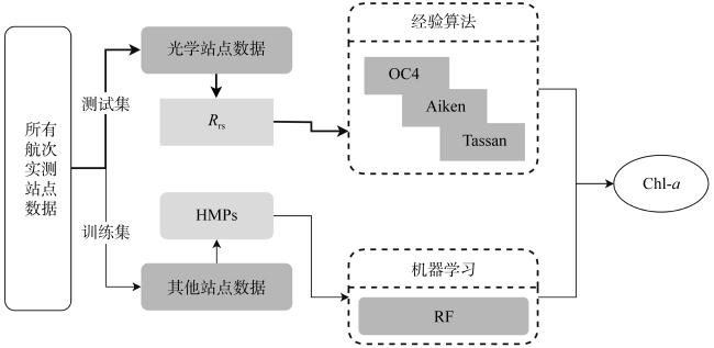
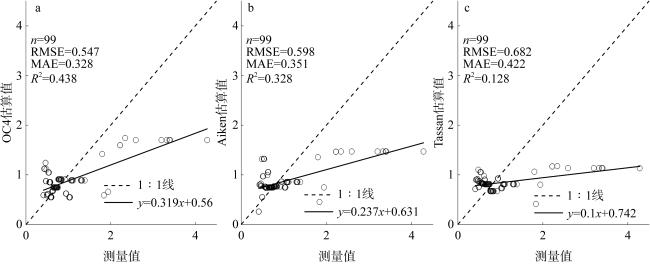
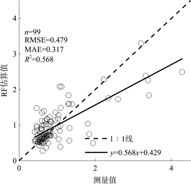
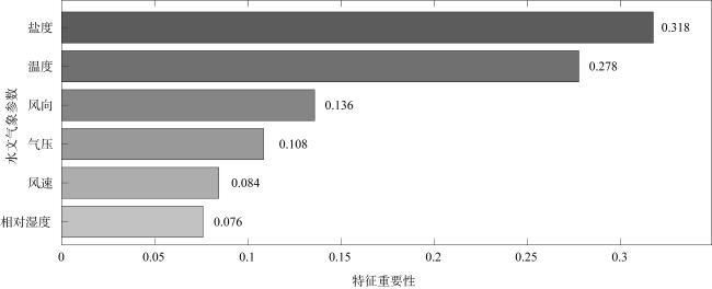
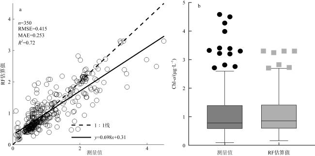
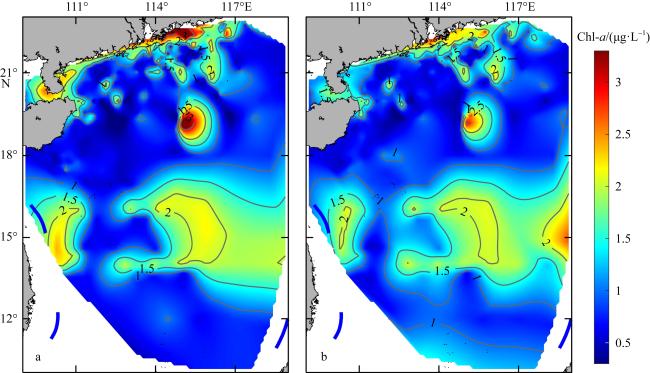
With the goal of low-cost and high-accuracy estimation of Chlorophyll-a (Chl-a), a model for estimating Chl-a in the surface layer of the Western South China Sea (WSCS) was constructed in this study. Using the data from the WSCS cruises in the past ten years, and based on the influence of changes of hydro-meteorological conditions and their contribution to the oceanic biochemical processes, the hydro-meteorological parameters (HMPs) were used as the input data of the random forest (RF) algorithm. To evaluate the reliability of estimating Chl-a based on HMPs, the quasi-analytical algorithm (QAA) was used to derive the in-situ remote sensing reflectance (Rrs) based on the measured inherent optical property parameters. Then Chl-a was estimated and evaluated by the combination of classical empirical algorithms for water color products such as Ocean Color 4 (OC4), Aiken and Tassan, and the evaluation results showed that the OC4 algorithm had the highest estimation accuracy, with an R2 of up to 0.438. The comparison with the R2 of 0.568 of the RF-based model shows that, owing to the large data volume of HMPs, the Chl-a estimation results of the RF model based on HMPs show much better stability and generalization, and better spatial distribution consistency with the measured results. It was found in study of the importance of feature parameters that in the machine learning model for estimating Chl-a based on HMPs, salinity is the most important feature variable, followed in turn by temperature, wind and air pressure, and the lowest contributor is relative humidity.

Cite this article

ZHENG Yuanning , LI Cai , ZHOU Wen , XU Zhantang , SHI Zhen , ZHANG Xianqing , LIU Cong , ZHAO Jincheng . Estimation of Chlorophyll-a in the western South China Sea based on hydro-meteorological parameters*[J]. Journal of Tropical Oceanography, 2025 , 44(2) : 18 -29 . DOI: 10.11978/2024095
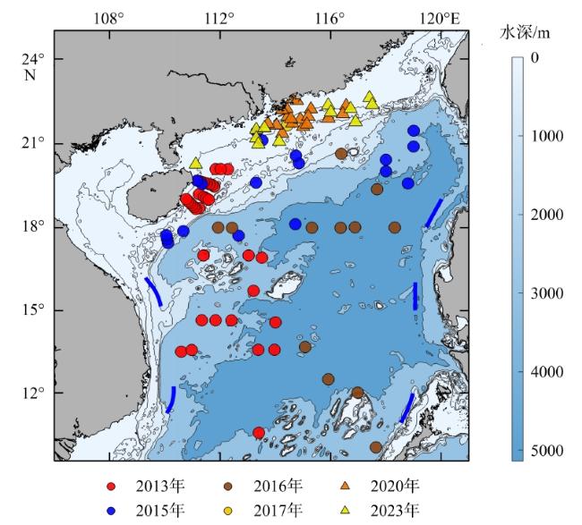
基于遥感反射率(remote sensing reflectance, Rrs)估算叶绿素a (Chlorophyll-a, Chl-a)浓度的经验算法已有大量研究。在水色卫星快速发展的推动下, 基于天基水色卫星的Rrs可以对Chl-a的时空分布进行研究分析。经验算法中, 一类水体的反演算法发展较为成熟且水域适应性和泛化性较好, 而二类水体水质较为复杂, 算法的区域适应性和泛化性较差(李建鸿 等, 2021; Caballero et al, 2022; Kwong et al, 2022), 在进行区域应用时还需结合实测数据对其进行本地化训练和适应。同时, 卫星图像易受气溶胶厚度、云层覆盖率及降雨等复杂边界条件影响, 高分辨率与大空间范围很难同时兼顾(Ma et al, 2021; Binh et al, 2022; Wang et al, 2023)。近些年, 基于无人机的光谱采样对天基水色遥感产品性能的提升起到了很好的补充作用(Chen et al, 2021), 利用空基光谱仪得到的高精度Rrs对天基Rrs进行校正, 以校正后的大时空尺度天基Rrs可以有效提升Chl-a经验算法的精度(Zhao et al, 2020)。除此之外, Rrs也可以通过水体固有及表观光学特性的经验及半分析算法模拟和估算得到(Cannizzaro et al, 2006; Lee et al, 2011; Loisel et al, 2017; Fu et al, 2020)。与遥感图像对环境条件要求较高不同, 基于水体固有及表观光学特性得到的Rrs可以避免天文气象条件对卫星系统成像的干扰, 但数据获取成本高。
水文气象作为水循环系统中重要的环境条件, 与水质变化息息相关, 水质变化过程受温盐深、流速流向以及风速、光照、降水量等水文气象参数(hydro-meteorological parameters, HMPs)的影响(Kotta et al, 2019; Garabaghi et al, 2023)。已有研究表明, 风是控制上升流和垂直混合深层水进入上层海洋的一个因素, 低温、高盐、高营养的深层水的垂直向上运动形成温度、盐度与Chl-a不同的剖面分布形态。同时, 风也影响海洋表面混合层深度, 在全球海洋中, 混合层较深的区域Chl-a与风速呈负相关, 而混合层较浅的区域Chl-a与风速呈正相关(Kahru et al, 2010)。盐度会影响营养物质对初级生产力的贡献, 海洋中陆源营养物质对Chl-a浓度的影响程度随着淡水富营养化程度的增加而增加(Sheng et al, 2023), 海洋中的富营养淡水输入, 风、潮汐等引起的物理运动, 影响Chl-a的分布特征并与区域内的温度和盐度差异紧密相关(Gao et al, 2008)。水文、气象传感器价格低廉, 操作简单。因此, 充分利用低成本测量的HMPs来构建水质估算模型是一个非常有前景的方法。
涉及概率论、统计学、逼近论、凸分析、算法复杂度理论等多门学科的机器学习具有操作简单和自适应性强的优点, 在解决海洋及其他领域不同参量之间的非线性关系上凸显出其独特的优势, 可以实现快速高精度的自适应估算模型的构建(Rahmani et al, 2021), 能够从大型和复杂的数据集中分析和提取特征, 而不依赖于明确的物理或化学方程(Zhi et al, 2024), 为基于水文气象等低成本参数估算水质参数提供了一种新的解决方案。
本文的研究区域位于中国南海西部海域(图1)。南海是沟通太平洋和印度洋, 联系亚洲、非洲和大洋洲的海上关键枢纽, 是新时代“一带一路”倡议的重要节点, 更是我国海洋强国战略实施的主战地。南海有富饶的生物资源和巨大的能源库, 厘清该海域水质环境可以科学指导蓝色经济的可持续发展以及海防安全体系构建。
图1 研究区域地图及2012、2013、2015—2020、2022和2023年南海航次数据站点位置

底图基于自然资源部标准地图服务网站下载的审图号为GS(2023)2762号的标准地图制作, 底图无修改

Fig. 1 Map of the study area and locations of sampling stations of the cruises in 2012, 2013, 2015-2020, 2022 and 2023 in the South China Sea

本文利用近十年南海区域实测HMPs、实测Chl-a浓度和水体固有光学特性参数, 研究了基于HMPs的Chl-a机器学习的最优化估算模型, 并将机器学习模型估算结果与基于Rrs经验算法估算结果进行对比分析, 以验证基于HMPs的Chl-a估算模型的可靠性和水域适应性。

1 数据来源及方法

1.1 数据

1.1.1 航次信息

本文中利用的航次站点覆盖了南海西部及海南岛东北部和受径流影响较大的珠江口水域。数据集包括2012、2013、2015—2020、2022和2023年的10 个调查航次(图1), 具体每年航次数据及其相关信息见表1。Chl-a的测量则采用了荧光测量法和基于水体固有光学特性的吸收线高度(absorption line height, aLH)法(Boss et al, 2013; Roesler et al, 2013) 。
表1 2012年至2023年12次巡航收集的信息概要

Tab. 1 A summary of the information collected from 2012 to 2023 on 12 cruises

年份 数据采集时间 覆盖范围 站点数
2012 9月30日—10月25日 14°00′—22°12′N, 110°12′—119°00′E 37
2013 8月9日—9月2日 10°00′—20°06′N, 110°30′—114°00′E 61
2015 6月21日—7月17日 17°24′—22°30′N, 109°30′—119°00′E 43
2016 9月3日—9月23日 10°00′—21°00′N, 111°30′—119°00′E 23
2017 10月1日—10月23日 18°24′—21°54′N, 110°18′—114°54′E 4
2018 6月12日—6月22日 21°30′—23°06′N, 113°12′—116°54′E 7
8月18日—8月25日 17°54′—21°18′N, 110°36′—115°18′E 1
2019 9月27日—10月5日 17°42′—23°00′N, 110°30′—117°06′E 3
2020 8月28日—9月4日 18°42′—22°00′N, 107°24′—117°00′E 32
6月1日—6月29日 17°24′—23°06′N, 110°00′—117°36′E 22
2022 8月14日—6月22 日 14°00′—22°24′N, 110°12′—119°00′E 27
2023 6月23日—7月20日 10°00′—20°06′N, 110°30′—114°00′E 129

1.1.2 叶绿素a

使用的Chl-a数据集中, 2022年和2023年的Chl-a数据是基于荧光传感器(fluorescence)获得的测量值, 简称为Chl-a (f)。受观测能力限制, 2012年、2013年和2015—2020年的Chl-a数据则是利用水体吸收衰减测量仪AC-9和AC-S 剖面观测的吸收系数 a ( λ ), 基于676nm处的吸收线高度计算得到的, 简称为Chl-a (aLH) (Zhang et al, 2023):
a BL z , 676 = a t w z , 715 a t w z , 650 715 650 ×           767 650 + a t w z , 650
a LH z , 676 = a t w z , 676 a BL z , 676
Chl - a a LH = A × a LH z , 676 B
式中: aBL(z, 676) 和aLH(z, 676) 分别表示676nm处的基线吸收值和吸收线高。at-w表示总吸收系数(total absorption coefficient, at)减去纯水吸收系数 (absorption coefficient of pure water, aw)。at-w(z, 715) 和 at-w(z, 650) 分别由AC-9和AC-S直接测量得到的。Chl-a (aLH)是根据aLH计算得出的Chl-a浓度。根据Deng等(2019)对南海区域的现场测量数据进行的回归, 公式(3)中AB表示幂函数的系数和指数, 分别为108.07和1.084。
为了比较两种测量方法得出的Chl-a, 利用2023年调查航次实测的Chl-a (f)以及利用现场ac-s实测的吸收系数估算得到的Chl-a (aLH), 根据测量站点的信息对测量数据进行了排列、整合和对比(图2~图5)。总体上, 两种方法得到的Chl-a的剖面变化曲线相似, 但C057站点的Chl-a (f)和 Chl-a (aLH)剖面变化趋势呈现出较大的差距(图 3)。对比分析二者的整个观测剖面数据(30m以浅)(图4a), 发现变化趋势是相似的。虽然它们的相关性在浅表层10~15m水体中不显著, 但将Chl-a (f)剖面分布的首尾相连时(黑色直线)可以看出两组数据具有明显的随剖面深度递增的变化趋势(图4b)。10m以浅二者之间差距较大, 究其原因可能是因为浅表层水环境过程变化快, 前后两次观测间隔时间长, 数据不同步所致。
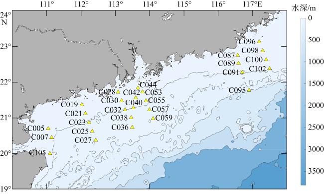
图2 具有Chl-a (f)和Chl-a (aLH)测量数据的2023年航次的站点分布图

底图基于自然资源部标准地图服务网站下载的审图号为GS(2023)2762号的标准地图制作, 底图无修改

Fig. 2 Location of stations for the 2023 cruise with Chl-a (f) and Chl-a (aLH) measurements
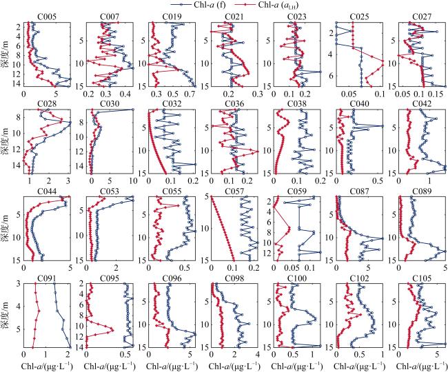
图3 两种方法在同一站点得到的测量结果对比

Fig. 3 The results of two types of measurements at the same stations

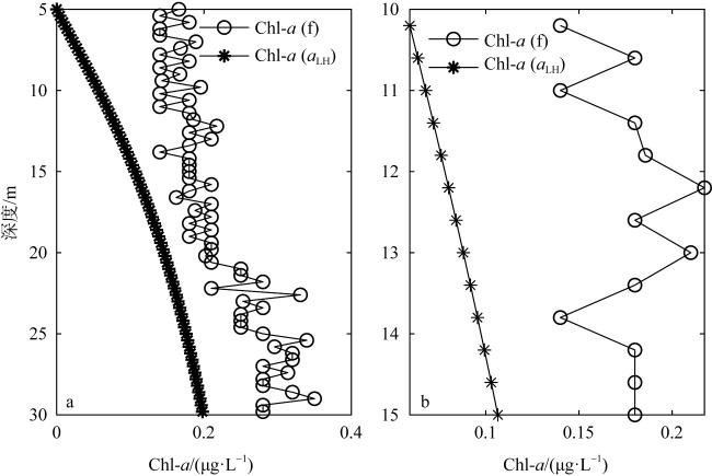
图4 C057站点的两组数据在5~30m (a)和10~15m (b)的变化曲线对比

Fig. 4 Comparison of the change curves of two measurements of data at 5~30 m (a) and 10~15 m (b) of the C057 station

图5 Chl-a (f) 与 Chl-a (aLH) 的拟合图(a)及Chl-a (f) 与调整后的Chl-a (aLH) 的对数拟合图(b)

Fig. 5 Fitting figure of Chl-a (f) and Chl-a (aLH) (a), fitting logarithmic figure of Chl-a (f) and adjusted Chl-a (aLH) (b)

Chl-a (aLH)与Chl-a (f)的拟合结果表明两者相关性好, 但数值范围差异较大(图5)。为了调整两种方法获取的Chl-a数值范围的差异, 研究过程中根据线性拟合公式(4)对 Chl-a (aLH) 数据进行了调整(图5b)。其中y为调整后的Chl-a (aLH), x为Chl-a (aLH)。
y = 1.631 x + 0.255

1.1.3 原位光学数据

本研究利用的水体光学特性参数来自2013、2015、2018和2023年的原位数据集。在调查期间具有水体光学特性参数采样的站点如图6所示, 匹配后共有99组水体光学特性参数。基于准分析算法(quasi-analytical algorithm, QAA)经验算法(Lee et al, 2011), 利用水体的吸收系数a( λ)与后向散射系数bb( λ)计算得到原位Rrs, 计算过程如下。
R rs = 0.52 r rs λ / 1 1.7 r rs λ
u λ = g 0 + g 0 2 + 4 g 1 × r rs λ 2 g 1
u λ = b b λ / a λ + b b λ
a = a w + a t w
b b = b bw + b bp
式中: r rs 是水面之下遥感反射率; g0g1为QAA算法给出的u( λ)和rrs( λ)经验公式中的系数, 分别是0.0089和0.1245。 b b 是由光谱后向散射仪Hydroscat-6测量获得的水体后向散射系数, 包括420nm、442nm、488nm、532nm、590nm、676nm 6个波段。 a w为常数, 对应以上6个波段的数值分别为0.00442、0.00696、0.0136、0.0434、0.1351、0.448 (Pope et al, 1997)。 b bp是海水颗粒物的后向散射系数, b bw是纯水的后向散射系数。
图6 固有光学特性数据站点图

底图基于自然资源部标准地图服务网站下载的审图号为GS(2023)2762号的标准地图制作, 底图无修改

Fig. 6 Map of the stations with data of inherent optical properties

1.1.4 水文气象参数

2023年Zheng等针对庙湾岛定点长时间序列底层水质参数估算研究发现, 与Chl-a相关性较高的6个HMPs分别为水温、盐度、气压、深度、相对湿度、风向(Zheng et al, 2024)。由于本研究中利用的Chl-a为5m水层的平面数据, 风速对水质因子的贡献不可忽视, 因此将风速补充为第6个参数。水温、盐度和水深等水文数据是在航行中由Seabird Electronics SBE-911的温盐深(conductivity temperature depth, CTD)仪器测量得到。气象数据来自欧洲中期天气预报中心(European Center for Medium-Range Weather Forecasts, ECMWF)对1950年1月至今全球气候的第五代大气再分析数据集(ECMWF Reanalysis v5, ERA5)中的每小时数据集(https://cds.climate.copernicus.eu), 空间分辨率为0.25° × 0.25°, 风速和风向由数据集中的uv分量计算得到。

1.2 方法

1.2.1 经验算法

为了将机器学习结果与经验算法的估算精度进行比较, 本文选用了目前应用较多的3种经验公式: 1) 是由O’Reilly等(1998)提出的, 以蓝绿波段比值对应不同Chl-a浓度为基础建立的, 能够适用于多种水体类型的海洋颜色(ocean color, OC)系列算法。根据不同阶的估算精度, 本研究中选择的是精度较高的OC4; 2) 是Aiken在1994年针对SeaWiFS卫星提出的Aiken经验算法, 该算法在我国东海与黄海的Chl-a估算中有较好的适应性(Siswanto et al, 2011); 3) 由于本研究使用的原位光学数据多分布在南海寡营养区(图6), 所以选取在地中海寡营养海域具有良好的适用性的Tassan算法, 该算法在我国黄海、东海的Chl-a估算中也取得了较高的估算精度(Gitelson et al, 1996; Siswanto et al, 2011)。通过MATLAB拟合方程确定经验算法的区域性最佳常数, 具体公式与利用参数见表2
表2 本研究中利用的经验算法简介

Tab. 2 Summary of empirical formulas used in this study

算法名称 算法公式 参数值 文献来源
OC4 M = log 10 max R rs λ blue R rs λ green
M = log 10 max R rs λ blue R rs λ green
R rs λ blue = R rs 442 nm;
a0=3.562; a1=-13.144; a2=15.409; a3=-5.997; a4=0.4
O’Reilly等(2019)
Aiken M = log R rs 488 nm R rs 532 nm
M = log R rs 488 nm R rs 532 nm
a0= -0.395; a1=0.803; a2=-0.158; a3=-0.118 Aiken等(1996)
Tassan M = r rs 442 nm r rs 532 nm r rs 420 nm r rs 488 nm a 0
M = r rs 442 nm r rs 532 nm r rs 420 nm r rs 488 nm a 0
a0=-1.012; a1=-0.439; a2=0.713; a3=-0.176 Tassan (1994)

注: R rs λ blue表示蓝光波段的遥感反射率, R rs λ green表示绿光波段的遥感反射率。在本文中442nm对应蓝光波段, 532nm对应绿光波段。 R rs λ 442表示442nm处的遥感反射率, R rs 532 nm表示532nm处的遥感反射率, R rs 488 nm表示448nm处的遥感反射率。 r rs 442 nm r rs 420 nm r rs 532 nm r rs 488 nm分别表示442nm、420nm、532nm、488nm处的水面之下遥感反射率。M表示不同经验算法中使用的波段比值变量, a0, a1, a2, a3, a4均为经验公式中的常数代称

1.2.2 机器学习算法

2023年Zheng等(2024)对庙湾岛的研究发现, 随机森林(random forest, RF)在基于HMPs估算水质参数中表现出显著的优势。基于此, 本研究利用的机器学习算法是随机森林, 其强大的数据处理能力在全球海洋过程研究和应用中已被证明是估算水质参数的有力工具(柳青青 等, 2021; Wang et al, 2021; 王春玲 等, 2022)。RF是bagging算法的一种扩展形式, 由多个决策树组成, 这些决策树基于bootstrap aggregating随机选择的子集构建(Breiman, 2001), 在构建决策树的过程中, 算法会随机选择样本及其相应的特征, 这种随机选择过程增强了基学习器的多样性, 提高了算法的泛化能力。
通过对航次Chl-a和HMPs的匹配, 最终形成的数据集中有350个站点, 为验证机器学习算法的精度, 研究中以公式(5)推导的原位Rrs对应站点数据(99条)组成测试集, 其他站点信息(251条)则用于建立RF模型的训练集。研究中, RF回归利用scikit-learn中的网格搜索(GridSearchCV)五折交叉验证进行模型超参数的确定(表3)。
表3 本研究中利用的随机森林算法的超参数

Tab. 3 Hyper-parameters of RF algorithm used in this study

算法 超参数 含义 设置值
RF n_estimators 决策树个数 3
max_depth 决策数的最大深度 7
random_state 随机种子 90

1.2.3 精度评价指标

采用均方根误差(root-mean-square error, RMSE)、平均绝对误差(mean absolute error, MAE)和决定系数(R2)作为指标, 评估模型的估算精度。RMSE、MAE 和 R2 的公式定义如下。
RMSE = 1 n i = 1 n y i y ^ i 2
MAE = 1 n i = 1 n y i y ^ i
R 2 = 1 i = 1 n y i y ^ i 2 i = 1 n y i y ¯ i 2
式中: n为样本量, y i为实测值, y ^ i为估算值。

1.2.4 归一化

为消除量纲引起的不同特征变量的数量级差异对模型分析结果的影响(张莹 等, 2019; Zhang et al, 2019), 研究过程中对所有输入数据进行了归一化处理。
X = x   x min x max x min
式中: X是归一化后的值, x是原始值, x max x min分别是原始数据中的最大值和最小值。

1.2.5 技术流程

研究流程依次包括原位Rrs结合经验算法进行Chl-a的估算, 和利用HMPs作为输入时, 结合RF算法进行建模。具体的技术流程见图7
图7 技术流程图

Fig. 7 Technique flowchart

2 结果

2.1 基于遥感反射率的估算

从评价指标的结果来看, 3种经验算法得到的Chl-a的估算精度均比较低, 但OC4算法的估算表现最好, R2达到了0.438 (图8a)。3种算法都在Chl-a的高值部分出现明显的低估, 推测是因为本研究中利用的Rrs数据量级差别较大导致的, 研究中利用的光学数据覆盖了南海大部分区域, 沿岸地区因为长期的人类活动污染, 具有较高的Chl-a, 但南海盆地地区是寡营养区, Chl-a较低, 二者之间有较为明显的水色差异(He et al, 2019), 经验算法对于这些差异没有表现出良好的兼容性。
图8 各经验算法基于Rrs得到的Chl-a的测量值和估算值的对比散点图

a. 基于OC4经验算法的估算值与测量值对比; b. 基于Aiken 算法的估算值与测量值对比; c. 基于Tassan算法的估算值与测量值对比

Fig. 8 Scatterplots of the measured and estimated Chl-a by empirical formulas based on Rrs

2.2 基于水文气象参数的估算

对比OC4与RF估算结果的散点图, 能够明显看出RF模型对于Chl-a值的变化有更强的适应能力(图9)。RF估算结果的精度评价指标RMSE、MAE和R2分别是0.479、0.317和0.568, 拟合线与1∶1线之间的距离也更小。在散点图中, 仅有少数站点在Chl-a高值部分出现了低估的现象, 并且低值部分在拟合线的散点密集程度也高于OC4的估算结果。
图9 RF基于HMPs得到的Chl-a的测量值和估算值的对比散点图

Fig. 9 Scatterplots of the measured and estimated Chl-a by the RF model based on HMPs

3 讨论

3.1 水文气象参数在RF模型中的特征重要性

特征重要性用于快速确定不同特征输入参数对模型计算结果所做的贡献(Cappelli et al, 2023)。特征的重要性越高, 意味着该特征对目标变量的影响越大(Wang et al, 2023)。RF算法本身包含一个用于评估数据拟合后特征重要性的指标, 在scikit-learn库中, 该指标被封装在RF算法的"feature_importances"参数中, 生成一个NumPy数组对象来量化每个特征的重要性(Yuan et al, 2023)。在特征重要性数组中, 数值越高表明相应的特征变量对提高数据集的精度贡献越大, 也充分突显出该特征的重要性。
以基于HMPs构建的RF模型为基础, 引入特征重要性来评估每个水文气象特征输入参数在Chl-a估算中的重要性。如图10所示, 依据重要性排序, 温度和盐度是对南海西部表层Chl-a变化过程影响最大的两个变量, 而相对湿度对Chl-a的影响程度小。
图10 每个水文气象参数在RF模型中的特征重要性

Fig. 10 The feature importance of individual HMPs in the RF model

3.2 基于RF模型的南海西部Chl-a的估算

图1中所有匹配站点的HMPs作为输入数据, 利用3.2节建立的RF模型对南海西部的Chl-a进行估算。估算结果相对于实测值的RMSE、MAE和R2分别为0.415、0.253和0.72 (图11a)。在最小值区域的散点分布显示RF模型表现了轻微的高估, 在Chl-a大于3μg·L-1的区域有明显的低估现象。从箱型图也能够明显看出, 实测数据中的大量高值在RF估算中出现了低估(图11b), 但数据中值区域的拟合效果较好, 图11a中黑色1∶1线附近的散点密集程度高。这说明RF与OC4算法都有对数据的极值变化的响应较差的缺点, 但相对于偏差较大的OC4算法, 通过在高值区域1∶1线条上的散点密度看出RF有更好的适应性。
图11 RF模型基于HMPs在完整数据集上的估算表现(a)和Chl-a的测量值与RF估算值的箱型图对比(b)

Fig. 11 The performance of the RF model on the whole dataset based on HMPs (a), and the comparison of box charts of measured and estimated Chl-a (b)

Chl-a的空间分布进一步表明RF估算结果在高值区域出现明显的低估, 特别是在珠江口流域, 但RF得到的Chl-a在整体的平面分布规律上与实测数据基本一致(图12)。珠江口Chl-a整体偏高, 且随着离岸距离呈递减趋势。这一分布主要归因于珠江口流域由于珠江附近的城市工业发达, 人口密集, 陆源污染严重, 所有调查数据基本集中在丰水期, 降雨、径流等作用使汇入南海的淡水携带大量营养物质(Sheng et al, 2023)。南海西部与海南岛东部附近海域Chl-a的高值主要是由于夏季西南季风引起的上升流过程使深水层富含营养物质的高盐度低温水向浅表层移动, 造成表层Chl-a升高(Huynh et al, 2020; Li et al, 2023)。在(18°N, 115°E)处, 气旋涡(冷涡)作用使该海域Chl-a有明显的抬升(Wu et al, 2017)。南海东部的西南季风在10月初结束, 在10月中下旬的站点采样期间, 逐渐强烈的东北季风使沿岸高Chl-a向西扩散(Xian et al, 2012; Matsumoto et al, 2020)。这些人为和自然条件使Chl-a发生变化的同时均伴随着明显的温度、盐度变化, 且上述过程与海面风的作用紧密相关。综上所述, 在南海西部及海南岛东部, 风引起的物理过程伴随着海水中的温度、盐度、Chl-a变化, 在珠江口, 淡水输入过程盐度变化最为明显, 因此, 温、盐变量是对RF模型估算Chl-a过程中贡献最高的特征参数, 而其他变量的相关性相对较低。
图12 Chl-a的测量值(a)与RF模型基于全部HMPs得到的Chl-a估算值(b)的平面分布

底图基于自然资源部标准地图服务网站下载的审图号为GS(2023)2762号的标准地图制作, 底图无修改

Fig. 12 The planar distribution of measured Chl-a (a) and estimated Chl-a (b) from the RF model based on the input of all HMPs

4 小结

本文以利用低成本获取得到的HMPs估算海表层Chl-a为目标, 借助先进的RF机器学习算法, 结合已有的QAA和OC4、Aiken、Tassan等经验算法, 研究了基于HMPs的Chl-a机器学习的最优化估算模型, 并将机器学习模型估算结果与基于Rrs经验算法估算结果进行对比分析, 以验证基于HMPs的Chl-a估算模型的可靠性和水域适应性。
研究基于近十年南海西部实测水体固有光学特性参数, 利用aLH方法估算得到的Chl-a (aLH)与荧光测量结果Chl-a (f)进行对比、校正、统一, 在此基础上, 以实测HMPs和Chl-a为特征参数, 利用RF为机器学习算法, 构建了基于HMPs的Chl-a估算模型。同时, 基于近十年南海西部实测水体固有光学特性数据, 利用QAA经验算法估算得到Rrs, 并以此为基础参数, 选择OC4、Aiken、Tassan等在我国海域应用较多的经验算法, 对调查海域的Chl-a进行估算及对比分析, 结果表明OC4算法的估算精度最高。将RF模型与OC4算法的估算结果进行对比发现, 基于OC4算法得到的Chl-a整体低估, 而基于HMPs建立的RF模型估算精度与实测Chl-a的平面分布吻合度较高。
研究还同时发现, 基于HMPs构建的Chl-a估算模型中, 盐度对RF估算模型的贡献最大, 温度次之, 贡献较小的为风向、气压和风速, 相对湿度的贡献度最低。实测及估算结果均表明, 珠江口及南海西部和海南岛东北部海域均呈现Chl-a高值, 这一分布主要受温盐及风速影响所致。
[1]
李建鸿, 黄昌春, 查勇, 等, 2021. 长江干流表层水体悬浮物的空间变化特征及遥感反演[J]. 环境科学, 42(11): 5239-5249.

LI JIANHONG, HUANG CHANGCHUN, ZHA YONG, et al, 2021. Spatial variation characteristics and remote sensing retrieval of total suspended matter in surface water of the yangtze river[J]. Environmental Science, 42(11): 5239-5249 (in Chinese with English abstract).

[2]
柳青青, 孟朔羽, 徐茗, 等, 2021. 随机森林反演卫星遥感海表面盐度研究[J]. 武汉大学学报(信息科学版), 48(9): 1538-1545.

LIU QINGQING, MENG SHUOYU, XU MING, et al, 2021. Satellite sea surface salinity retrieval using random forest model[J]. Geomatics and Information Science of Wuhan University, 48(9): 1538-1545 (in Chinese with English abstract).

[3]
王春玲, 史锴源, 明星, 等, 2022. 基于机器学习的水体化学需氧量高光谱反演模型对比研究[J]. 光谱学与光谱分析, 42(8): 2353-2358.

WANG CHUNLING, SHI KAIYUAN, MING XING, et al, 2022. A comparative study of the cod hyperspectral inversion models in water based on the maching learning[J]. Spectroscopy and Spectral Analysis, 42(8): 2353-2358 (in Chinese with English abstract).

[4]
张莹, 谢仕义, 邓伟彬, 等, 2019. 基于机器学习理论的海洋水质评价模型[J]. 物探化探计算技术, 41(6): 819-825.

ZHANG YING, XIE SHIYI, DENG WEIBIN, et al, 2019. Ocean water quality evaluation model based on machine learning theory[J]. Computing Techniques for Geophysical and Geochemical Exploration, 41(6): 819-825 (in Chinese with English abstract).

[5]
AIKEN J, MOORE G F, TREES C C, et al, 1996. The SeaWiFS CZCS-type pigment algorithm[J]. Oceanographic Literature Review, 43(3): 315-316.

[6]
BINH N A, HOA P V, THAO G T P, et al, 2022. Evaluation of Chlorophyll-a estimation using Sentinel 3 based on various algorithms in southern coastal Vietnam[J]. International Journal of Applied Earth Observation and Geoinformation, 112: 102951.

[7]
BOSS E, PICHERAL M, LEEUW T, et al, 2013. The characteristics of particulate absorption, scattering and attenuation coefficients in the surface ocean; Contribution of the Tara Oceans expedition[J]. Methods in Oceanography, 7: 52-62.

[8]
BREIMAN L, 2001. Random forests[J]. Machine Learning, 45(1): 5-32.

[9]
CABALLERO I, ROMÁN A, TOVAR-SÁNCHEZ A, et al, 2022. Water quality monitoring with Sentinel-2 and Landsat-8 satellites during the 2021 volcanic eruption in La Palma (Canary Islands)[J]. Science of the Total Environment, 822: 153433.

[10]
CANNIZZARO J P, CARDER K L, 2006. Estimating chlorophyll a concentrations from remote-sensing reflectance in optically shallow waters[J]. Remote Sensing of Environment, 101(1): 13-24.

[11]
CAPPELLI F, GRIMALDI S, 2023. Feature importance measures for hydrological applications: insights from a virtual experiment[J]. Stochastic Environmental Research and Risk Assessment, 37(12): 4921-4939.

[12]
CHEN BOTAO, MU XI, CHEN PENG, et al, 2021. Machine learning-based inversion of water quality parameters in typical reach of the urban river by UAV multispectral data[J]. Ecological Indicators, 133: 108434.

[13]
DENG LIN, ZHOU WEN, CAO WENXI, et al, 2019. Retrieving phytoplankton size class from the absorption coefficient and chlorophyll a concentration based on support vector machine[J]. Remote Sensing, 11(9): 1054.

[14]
FU DONGYANG, HUANG YUYE, LIU DAZHAO, et al, 2020. Analysis of the regional spectral properties in northwestern South China Sea based on an empirical orthogonal function[J]. Acta Oceanologica Sinica, 39(7): 107-114.

[15]
GAO SHAN, WANG HUI, 2008. Seasonal and spatial distributions of phytoplankton biomass associated with monsoon and oceanic environments in the South China Sea[J]. Acta Oceanologica Sinica, 27(6): 17-32.

[16]
GARABAGHI F H, BENZER S, BENZER R, 2023. Modeling dissolved oxygen concentration using machine learning techniques with dimensionality reduction approach[J]. Environmental Monitoring and Assessment, 195(7): 879.

DOI PMID

[17]
GITELSON A, KARNIELI A, GOLDMAN N, et al, 1996. Chlorophyll estimation in the Southeastern Mediterranean using CZCS images: adaptation of an algorithm and its validation[J]. Journal of Marine Systems, 9(3-4): 283-290.

[18]
HE QINGYOU, ZHAN HAIGANG, XU JIE, et al, 2019. Eddy-induced chlorophyll anomalies in the Western South China Sea[J]. Journal of Geophysical Research: Oceans, 124(12): 9487-9506.

[19]
HUYNH H N T, ALVERA-AZCÁRATE A, BECKERS J M, 2020. Analysis of surface chlorophyll a associated with sea surface temperature and surface wind in the South China Sea[J]. Ocean Dynamics, 70(1): 139-161.

[20]
KAHRU M, GILLE S T, MURTUGUDDE R, et al, 2010. Global correlations between winds and ocean chlorophyll[J]. Journal of Geophysical Research: Oceans, 115(C12): C12040.

[21]
KOTTA D, KITSIOU D, 2019. Chlorophyll in the eastern Mediterranean sea: correlations with environmental factors and trends[J]. Environments, 6(8): 98.

[22]
KWONG I H Y, WONG F K K, FUNG T, 2022. Automatic mapping and monitoring of marine water quality parameters in Hong Kong using sentinel-2 image time-series and google earth engine cloud computing[J]. Frontiers in Marine Science, 9: 871470.

[23]
LEE Z P, DU KEPING, VOSS K J, et al, 2011. An inherent-optical-property-centered approach to correct the angular effects in water-leaving radiance[J]. Applied Optics, 50(19): 3155-3167.

[24]
LI JUNYI, LI MIN, WANG CHAO, et al, 2023. Multiple mechanisms for chlorophyll a concentration variations in coastal upwelling regions: a case study east of Hainan Island in the South China Sea[J]. Ocean Science, 19(2): 469-484.

[25]
LOISEL H, VANTREPOTTE V, OUILLON S, et al, 2017. Assessment and analysis of the chlorophyll-a concentration variability over the Vietnamese coastal waters from the MERIS ocean color sensor (2002-2012)[J]. Remote Sensing of Environment, 190: 217-232.

[26]
MA CHUNLEI, ZHAO JUN, AI BIN, et al, 2021. Two-decade variability of sea surface temperature and chlorophyll-a in the Northern South China Sea as revealed by reconstructed cloud-free satellite data[J]. IEEE Transactions on Geoscience and Remote Sensing, 59(11): 9033-9046.

[27]
MATSUMOTO J, OLAGUERA L M P, NGUYEN-LE D, et al, 2020. Climatological seasonal changes of wind and rainfall in the Philippines[J]. International Journal of Climatology, 40(11): 4843-4857.

[28]
O’REILLY J E, MARITORENA S, MITCHELL B G, et al, 1998. Ocean color chlorophyll algorithms for SeaWiFS[J]. Journal of Geophysical Research: Oceans, 103(C11): 24937-24953.

[29]
O’REILLY J E, WERDELL P J, 2019. Chlorophyll algorithms for ocean color sensors - OC4, OC5 & OC6[J]. Remote Sensing of Environment, 229: 32-47.

[30]
POPE R M, FRY E S, 1997. Absorption spectrum (380-700 nm) of pure water. Ⅱ. Integrating cavity measurements[J]. Applied Optics, 36(33): 8710-8723.

[31]
RAHMANI F, LAWSON K, OUYANG WENYU, et al, 2021. Exploring the exceptional performance of a deep learning stream temperature model and the value of streamflow data[J]. Environmental Research Letters, 16(2): 024025.

[32]
ROESLER C S, BARNARD A H, 2013. Optical proxy for phytoplankton biomass in the absence of photophysiology: rethinking the absorption line height[J]. Methods in Oceanography, 7: 79-94.

[33]
SHENG CHONG, JIAO J J, LUO XIN, et al, 2023. Offshore freshened groundwater in the Pearl River estuary and shelf as a significant water resource[J]. Nature Communications, 14(1): 3781.

DOI PMID

[34]
SISWANTO E, TANG JUNWU, YAMAGUCHI H, et al, 2011. Empirical ocean-color algorithms to retrieve chlorophyll-a, total suspended matter, and colored dissolved organic matter absorption coefficient in the Yellow and East China Seas[J]. Journal of Oceanography, 67(5): 627-650.

[35]
TASSAN S, 1994. Local algorithms using SeaWiFS data for the retrieval of phytoplankton, pigments, suspended sediment, and yellow substance in coastal waters[J]. Applied Optics, 33(12): 2369-2378.

DOI PMID

[36]
WANG FEIER, WANG YIXU, ZHANG KAI, et al, 2021. Spatial heterogeneity modeling of water quality based on random forest regression and model interpretation[J]. Environmental Research, 202: 111660.

[37]
WANG TIANHAO, SUN YU, SU HUA, et al, 2023. Declined trends of chlorophyll a in the South China Sea over 2005-2019 from remote sensing reconstruction[J]. Acta Oceanologica Sinica, 42(1): 12-24.

[38]
WU MEILIN, WANG YOUSHAO, DONG JUNDE, et al, 2017. Spatial assessment of water quality using chemometrics in the Pearl River Estuary, China[J]. Frontiers of Earth Science, 11(1): 114-126.

DOI

[39]
XIAN TAO, SUN LIANG, YANG YUANJIAN, et al, 2012. Monsoon and eddy forcing of chlorophyll-a variation in the northeast South China Sea[J]. International Journal of Remote Sensing, 33(23): 7431-7443.

[40]
YUAN XIAOGUANG, LIU SHIRUO, FENG WEI, et al, 2023. Feature importance ranking of random forest-based end-to-end learning algorithm[J]. Remote Sensing, 15(21): 5203.

[41]
ZHANG XIANQING, LI CAI, ZHENG YUANNING, et al, 2023. Approach for estimating the vertical distribution of the diffuse attenuation coefficient in the South China Sea[J]. Optics Express, 31(26): 43771-43789.

DOI PMID

[42]
ZHANG YIFAN, FITCH P, VILAS M P, et al, 2019. Applying multi-layer artificial neural network and mutual information to the prediction of trends in dissolved oxygen[J]. Frontiers in Environmental Science, 7: 46.

[43]
ZHAO YANPING, SONG YUMEI, CUI JINLI, et al, 2020. Assessment of water quality evolution in the Pearl River estuary (South Guangzhou) from 2008 to 2017[J]. Water, 12( 1): 59.

[44]
ZHENG YUANNING, LI CAI, ZHANG XIANQING, et al, 2024. Estimation of water quality parameters based on time series hydrometeorological data in Miaowan Island[J]. Ecological Indicators, 159: 111693.

[45]
ZHI WEI, APPLING A P, GOLDEN H E, et al, 2024. Deep learning for water quality[J]. Nature Water, 2(3): 228-241.

Outlines

/