Orginal Article

The spectral characteristics of phytoplankton absorption coefficient and assessment of MODIS-Aqua products in typical sea areas of the South China Sea

  • ZHAO Wenjing , 1 ,
  • CAO Wenxi , 2 ,
  • HU shuibo 3 ,
  • WANG Guifen 2 ,
  • LIU Zhenyu 4 ,
  • XU Min 1
Expand
  • 1. South China Institute of Environmental Sciences, the Ministry of Environmental Protection of RPC, Guangzhou 510535, China
  • 2. State Key Laboratory of Tropical Oceanography (South China Sea Institute of Oceanology, Chinese Academy of Sciences), Guangzhou 510301, China
  • 3. Shenzhen Key Laboratory of Spatial Information Smart Sensing and Services and Key Laboratory for Geo-Environment Monitoring of Coastal Zone of the National Administration of Surveying, Mapping and Geo-Information, Shenzhen University, Shenzhen 518060, China
  • 4. College of Resources and Environmental Science, South-central University for Nationalities, Wuhan 430074, China;
Corresponding author: CAO Wenxi. E-mail:

Received date: 2017-06-08

  Request revised date: 2017-08-15

  Online published: 2018-05-03

Supported by

National Natural Science Foundation of China (41506202)

Natural Science Foundation of Guangdong Province (2014A030310287)

State Key Laboratory of Tropical Oceanography Under Independent Project (LTO1509)

Project of Basic Scientific Research Expenses Supported by the Central Public Welfare Research Institute (South China Institute of Environmental Sciences, Ministry of Environmental Protection, PM-zx703-201601-014)

Ministry of Environmental Protection department budget Project (The policy research of coastal areas pollution prevention and control technology)

Science and Technology Planning Project of Guangxi (AB16380339)

Natural Science Foundation of Hubei Province (BZY15028)

Copyright

热带海洋学报编辑部

Abstract

Using remote sensing to accurately estimate phytoplankton absorption coefficient aph(l) can provide basic data and useful method to distinguish different functions of phytoplankton species for long time and large spatial scale. In this paper, the characteristics of aph(l) spectral are compared and analyzed in four typical areas of the South China Sea (SCS), east area of Qiongdong (QD), Guangdong Coastal area (GD), and the Pearl River Estuary (PE) by using field data collected during2003-2012.Then, the phytoplankton population structure differences are preliminarily identified. Furthermore, the performances of MODIS-Aqua aph(l) products derived from the semi-analytical algorithm QAA and empirical algorithm PL by using MODIS-Aqua remote sensing reflectance Rrs(l) products are compared in the SCS and QD waters based on the relaxed match-ups between MODIS-Aqua products and field data. The results show the differences of aph(l) spectral features are obvious among the clear water represented by the SCS and QD and turbid waters represented by GD and PE. In the clear waters, the aph(l) value is small but in a dominant position of particle absorption, while in the GD and PE areas, the aph(l) value is relatively large but not in a dominant position. The aph(l) coefficient have obvious spatial differences, and the possible causes are pigment packaging effect and the variation of pigment composition and concentration. MODIS-Aqua aph(l) products derived from the empirical algorithm PL perform better than those from the semi-analytical algorithm QAA. The algorithm QAA-derived aph(l) products underestimate the results compared to the field data, while the algorithm PL overestimate the results, with the average relative error (APD)less than 22% for both algorithms. There is a great improvement in the accuracy of the PL algorithm by using the Chl-a products derived from the optimized algorithm of OCI (named algorithm NOCI), with the APD less than 14%. In summary, there are strong application prospects to discuss different functions of ocean phytoplankton species by using remote sensing products.

Cite this article

ZHAO Wenjing , CAO Wenxi , HU shuibo , WANG Guifen , LIU Zhenyu , XU Min . The spectral characteristics of phytoplankton absorption coefficient and assessment of MODIS-Aqua products in typical sea areas of the South China Sea[J]. Journal of Tropical Oceanography, 2018 , 37(3) : 35 -44 . DOI: 10.11978/2017067

浮游植物在浮游食物网和海洋地球化学循环中发挥非常重要的作用。在大洋一类水体中, 浮游植物是总悬浮颗粒物吸收光谱的主要贡献者, 浮游植物吸收光谱受到多种因素如浮游植物种群结构、光照、营养盐等环境参数的影响而表现不同的变化规律(Bricaud et al, 1998); 浮游植物光谱吸收系数(aph(l))与叶绿素a浓度(Chl-a)的比值, 即浮游植物单位吸收系数(a*ph(l)), 其变化反映了浮游植物种群结构的差异; 因此, 浮游植物吸收光谱形状变化是基于水色遥感信号辨别不同浮游植物功能种群重要的生物-光学指针之一(Aiken et al, 2007, 2008)。
近年来, 随着多种形式固有光学参数水色遥感算法的构建和优化, 为基于水色遥感数据反演浮游植物种群信息变化奠定了扎实的基础。固有光学参量反演模型逐步从传统的经验统计模型深入到半分析模型, 经验模型是通过对固有光学参量与辐照度反射比或遥感反射率(R(l)或Rrs(l))进行一次或多次回归获得, 具有算法形式简单、处理速度快等优点; 半分析模型则是通过辐射传输方程建立表观光学量与固有光学量之间的关系, 具有物理意义明确、实用性强、反演精度高等特点。
国内外很多学者针对不同海区发展了许多经验模型。Lee等(1998)年建立了一种估算440nm波段的总吸收系数和色素吸收系数的经验算法。王桂芬(2008)基于2003—2007年5个航次的观测数据, 建立了南海北部海域总颗粒物、浮游植物、无机颗粒物吸收系数的经验反演模式。与此同时, Lee等(2007)、Carder等(1999, 2004)、Loisel等(2000, 2001)在不同海区构建有不同形式的半分析算法, 其中, Lee等(2007)构建的QAA半分析算法(quasi-analy-tical algorithm)应用最为深入和广泛。国内学者Qing等(2012)利用现场实测数据检验了QAA算法在黄海的适用性; 汪文琦等(2009)利用该算法对南海和福建沿岸水体吸收系数进行了反演; 郝艳玲等(2011)对珠江口赤潮水体的适用性上也进行了深入分析。
随着大量长时间序列、高质量实测数据的积累, 全面分析南海各典型海区aph(l)光学特性, 进一步评估主流卫星遥感产品对aph(l)产品的反演精度, 对于深入了解南海各典型海区的浮游植物种群结构、生物环境特性具有重要意义。本文利用2003年至2012年获取自南海、琼东为代表的清洁海域和以广东沿岸、珠江口为代表的浑浊海域的生物光学数据集, 开展南海各典型海区aph(l)光谱特征分析和讨论; 针对国际主流水色传感器MODIS-Aqua, 对比分析经验算法与半分析算法在反演南海aph(l)产品的差异, 同时给出算法优化建议, 以更好地为本地区海洋地球生物化学研究服务。

1 数据与方法

1.1 现场实验

2003年至2012年, 南海各典型海区共获取了9个航次的生物光学观测数据。其中, 南海开阔海区(SCS)和琼东海区(QD)数据获取时间为2004—2012年, 广东省沿岸(GD)和珠江口(PE)海区数据获取时间分别为2003和2007年, 为同步分析a*ph(l)在各典型海区的变化情况, 本文选取aph(l)与Chl-a现场观测相匹配的数据集, 南海各典型海域空间位置及实测站点分布见图1, 上述各典型海区实测匹配数据分别为170、58、23和10组。
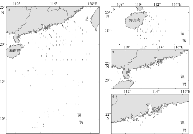
Fig. 1 Typical area of the South China Sea (SCS), and spatial distribution of in situ aph(l) data (open circles).The dots represent the spatial distribution of relaxed (cross) match-ups for MODIS-Aqua Rrs(l) and aph(l). (a) The open sea of the SCS; (b) the coastal area of Qingdong (QD); (c) the coastal area of Guangdong (GD); and (d) the Pearl River Estuary (PE)

图1 2004—2012年南海各典型海区位置及aph(l)现场观测站位(空心圆圈表示)空间分布示意
a. 南海开阔海区; b. 琼东海区; c. 广东沿岸; d. 珠江口。实心圆点表示宽松匹配法则下MODIS-Aqua Rrs(l)产品与实测aph(l)匹配数据的空间分布

浮游植物Chl-a和浮游植物色素的光谱吸收系数测量分为现场水样获取和实验室处理两个步骤。首先, 利用Niskin采水器分别采集标准层深度的海水, 在低真空度(小于5.96kPa)压力下分别将一定体积(2~4L)的水样过滤到直径25mm、孔径0.7μm的Whatman GF/F滤膜上, 保存在液氮生物容器中。带回实验室后, Chl-a采用Turner-Design10型荧光光度计进行测量, 有关测量方法可参见Parsons等(1984)。总悬浮颗粒物吸收光谱ap(λ)利用双光束紫外可见光分光光度计进行测量, 详细的测量过程参考文献(赵冬至等, 2004)。南海各典型海区(SCS、QD、GD和PE)的Chl-a浓度范围分别为0.03~3.25、0.03~0.16、0.16~18.16和0.58~25.60mg·m-3

1.2 遥感数据

本文利用的卫星数据是空间分辨率为1km的MODIS-Aqua业务化二级遥感产品, 该传感器自2002年发射至今可持续稳定地提供数据。传感器的中心波长为412、443、488、531、551和667nm, 除412nm中心波长的波段宽度为15nm之外, 其余中心波长的波段宽度均为10nm。辐射产品所采用的大气校正方法是Gordon等(1994)以及Wang(2005)后续优化的方法; Chl-a业务化二级产品采用的方法是O'Reilly等(2000)所提出的波段比值算法OC3, 最近Hu等(2012)针对低Chl-a水体提出了新的算法OCI, 在多清洁海区应用并取得良好效果。
参照国际上普遍采用的遥感产品检验标准和流程(Bailey et al, 2006), 考虑到南海典型海区实测与卫星匹配数据对的有限性, 为引入更多的统计样本, 增加统计结果的可信度, 本文按照Cui等(2010)对于宽松匹配法则的设定方法, 将时间窗口扩大至当天(±14h)。上述匹配法则已在南海和琼东海域评估MODIS-Aqua遥感产品中表明是可行的、评估结果是可信的(赵文静, 2014; Zhao et al, 2014)。经处理, 广东沿岸与珠江口海域无现场观测与遥感产品匹配数据, 南海和琼东海域的MODIS-Aqua Rrs(l)产品与相应现场观测获得的aph(l)匹配数据集共23组。其中, 琼东海域4组, 南海海域共19组。

1.3 浮游植物吸收系数反演算法

1.3.1 Prieur和Lee经验算法(以下简称PL算法)
Prieur等(1981)提出了aph(440)与Chl-a浓度CChl的经验关系如下:
aph(440)=A×CChlB
其中AB的取值分别为0.06和0.65。
Lee等(1998)建立了440nm处浮游植物吸收系数和其他波段处系数之间的关系:
aph(l)={a0(l)+a1(l)ln[aph(440)]}×aph(440)
采用公式(1)估算获得aph(440), 再利用公式(2)估算其他波段的吸收系数。本研究将440nm全部替换为443nm, a0(l)与a1(l)表示随波长变化的系数。
1.3.2 QAA半分析模型
QAA算法(Lee et al, 2007)可分为两个部分: 第一部分反演获得总吸收系数和颗粒物后向散射系数; 第二部分将总吸收系数再分解为浮游植物色素吸收系数aph(λ)及黄色物质和碎屑的吸收系数adg(λ)。大洋水体中, 参考波段通常选定为555nm, 本文计算结果具体选择的方法为QAA_v5 (http://www.ioccg. org/groups/Software_OCA/QAA_v5.pdf), 计算过程简述如下。
首先采用Gordon等(1988)模型, 通过Rrs(l)获得恰在水面之下的遥感反射率rrs(λ), 进而导出u(λ):
rrs(λ)=Rrs(l)/[0.52+1.7Rrs(l)]
rrs(λ)=g0u(λ)+g1[u(λ)]2
u(λ)={-g0+[g02+4g1rrs(λ)]0.5}/2g1
u(λ)=bb(λ)/[at(λ)+bb(λ)]
其中g0g1取值分别为0.0895和0.1247, bb(λ)为颗粒物后向散射系数, at(λ)为总吸收系数。
反演获得总吸收系数at(λ)和颗粒物后向散射系数bb(λ)后, 接下来需要将总吸收系数再分解为各个主要组分的吸收。因为在模拟过程中黄色物质和碎屑不容易分解开来, 所以公式(8)将adg(λ)作为一个独立的光学参数:
at(λ)=aw(λ)+aph(λ)+adg(λ)
aw(λ)为水体吸收系数; 黄色物质和碎屑颗粒物的吸收系数adg(λ)用一个随波长增加而减小的指数函数模拟(Roesler et al, 1989; Carder et al,1991), 如下式:
adg(λ)=adg(λ0)×exp[S×(λ-λ0)]
其中: adg(λ0)为黄色物质和碎屑颗粒物在参考波长λ0处的吸收系数; λ0为555nm; S为指数衰减常数, 它依赖于黄色物质类型的相对比例, 本文S值取0.015, 其他研究发现S指数系数通常介于0.014到0.019之间; aw(λ0)的取值参见Pope等(1997)所给的取值。

1.4 统计参数

本文选取均方根误差(RMS)、平均绝对误差(APD)、平均相对误差(RPD)、遥感产品值与实测值之比的中值(Ratio)、四分位(SIQR, semi-interquartile range)等指标来对上述算法结果进行评价; 斜率(slope)、截距(interception)、决定系数(R2)用来表征遥感产品值与实测值的线性拟合情况。上述参数均为线性坐标下的计算结果(Cui et al, 2010; 赵文静 等, 2014)。

2 结果与分析

2.1 南海典型海区水体浮游植物吸收光谱特征

南海各典型海区浮游植物色素吸收aph(λ)光谱如图2所示。
由图可见, 浮游植物色素吸收光谱呈明显的双峰形态分布, 443和670nm是浮游植物色素吸收作用较强的波段。南海开阔海域在443nm处的波峰值基本上小于0.12m-1; 琼东海域量值较小且较为集中, 介于0.005至0.02m-1之间; 广东沿岸和珠江口附近海域光谱类似, 670nm的峰值较高, 蓝光波段量值相对较大, 最大可达0.6m-1.
按照曹文熙等(2003)分类可知(图3), 南海和琼东海域属于典型的浮游植物色素吸收主导型, 总悬浮颗粒物吸收系数ap(λ)(指浮游植物色素吸收aph(λ)与非色素颗粒物吸收之和)光谱形状与aph(λ)光谱相似, 呈明显的双峰状; 而广东沿岸和珠江口海域ap(λ)光谱既有浮游植物色素主导型, 又有非色素颗粒物主导型, 总体上量值远大于南海和琼东海域。根据各海区aph(443)占ap(443)的比例来看, 广东沿岸海域为30%, 珠江口海域为58%, 而南海开阔和琼东海域分别高达76%和79%。
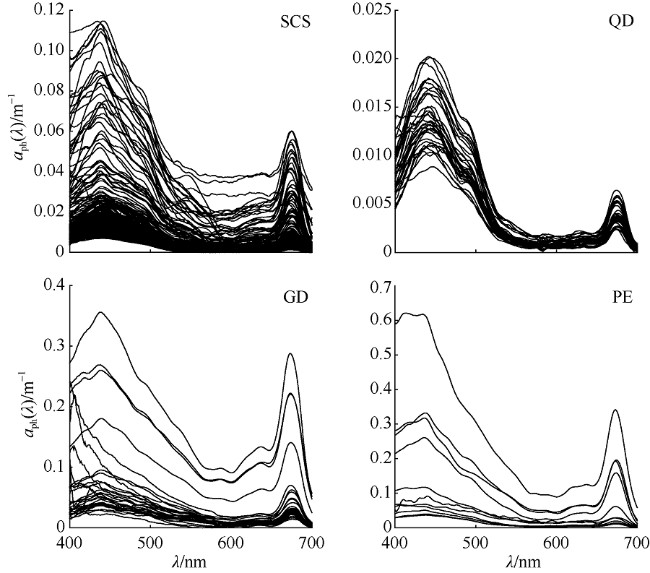
Fig. 2 In situ data spectra of aph(λ) in the SCS, QD, GD, and PE waters

图2 南海(SCS)、琼东(QD)、广东沿岸(GD)和珠江口附近海域(PE)水体浮游植物吸收aph(λ)光谱

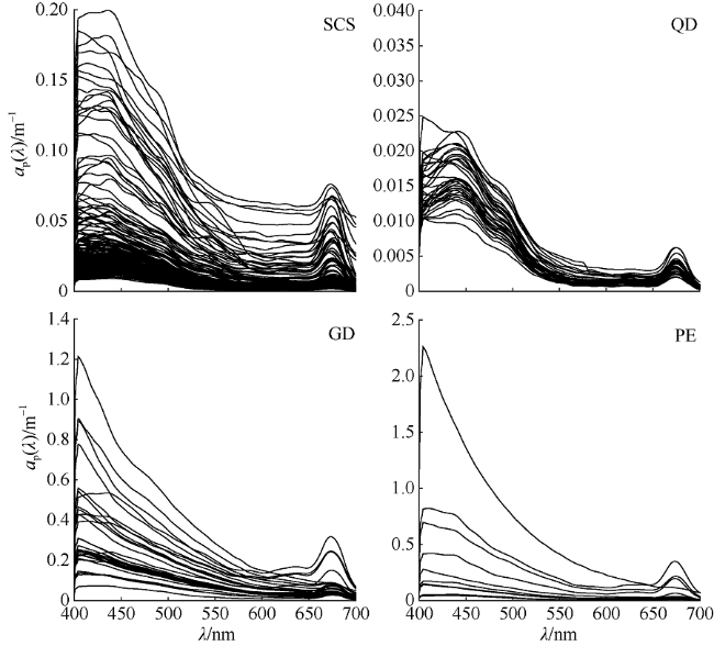
Fig. 3 In situ data spectra of ap(λ) in the SCS, QD, GD, and PE waters

图3 南海(SCS)、琼东(QD)、广东沿岸(GD)和珠江口附近海域(PE)水体颗粒物吸收ap(λ)光谱

南海各典型海区浮游植物单位吸收系数aph*(λ)光谱见图4表1, aph*(443)和aph*(667)随Chl-a变化情况见图5。总体来看, aph*(443)和aph*(667)在南海各典型海区各不相同。清洁的一类海区aph*(443)和aph*(667)明显大于浑浊的二类海区, 但各海区的aph*(667)在量值和变化幅度上均小于aph*(443), 这主要是因为443nm波段不仅有Chl-a的吸收, 也有其他吸收色素, 且aph*(443)色素打包效应高于aph*(667)。aph*(443)/aph*(667)量值较大意味着水体中附属色素的含量较多, 这表明南海和琼东海域水体中的附属色素较多(崔廷伟, 2006)。aph*(443)和aph*(667)随Chl-a浓度的变化均呈现明显的递减趋势, 但沿岸浑浊海域水体与清洁外海水体aph*(λ)变化趋势略有不同, 南海和琼东海域高单位吸收系数对应低Chl-a浓度, 琼东海域分布更集中; 而珠江口和广东沿岸海域则具有高Chl-a浓度和相对低的单位吸收系数, 这主要是由于不同水体中浮游植物种群结构不同而导致的(王桂芬, 2008)。
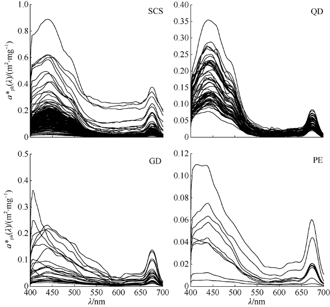
Fig. 4 In situ data spectra of aph*(λ) in the SCS, QD, GD, and PE waters

图4 南海(SCS)、琼东(QD)、广东沿岸(GD)和珠江口附近海域(PE)水体浮游植物单位吸收系数aph*(λ)光谱

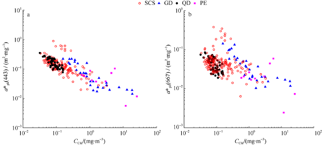
Fig. 5 Variations of aph*(443)(a) and aph*(667) (b) with CChl

图5 aph*(443)(a)和aph*(667)(b)分别随CChl的变化

Tab. 1 The ranges of aph*(443), aph*(667) and aph*(443)/ aph*(667) in each typical area of the SCS

表1 南海各典型海区单位吸收系数aph*(443), aph*(667)和aph*(443)/ aph*(667)量值范围

海区 aph*(443) aph*(667) aph*(443)/aph*(667)
南海 0.02~0.90 (0.16) 0.006~0.32 (0.05) 1.33~7.13 (3.85)
琼东 0.08~0.35 (0.17) 0.02~0.07 (0.04) 3.13~7.61 (4.81)
广东 0.01~0.22 (0.08) 0.008~0.11 (0.04) 1.15~4.52 (2.26)
珠江口 0.006~0.1 (0.05) 0.002~0.05 (0.02) 1.79~3.82 (2.58)

注: 表格中的数值格式为“最小值~最大值(平均值)”。

2.2 浮游植物吸收系数遥感估算的精度评估

2.2.1 基于遥感反射率产品, 采用QAA和PL算法的精度对比
基于MODIS-Aqua遥感反射率Rrs(λ)产品, 分别利用经验算法PL(Chl-a产品由业务化算法OC3反演获得)和半分析算法QAA, 获得的aph(λ)产品值与实测值之间的散点图如图6表2所示。其中, λ为412、443和490nm, 因为基于算法Lee获得的aph(λ)(λ>490nm)反演值多为负值。
图6可知, aph(λ)(λ=412, 443, 490)与相应实测值的散点图基本上位于1︰1线的两侧, 但QAA半分析算法得到的反演值相对于实测值存在明显的低估; 而经验算法PL得到的反演值和实测值更集中地分布在1︰1线的两侧, 产品值相对于实测值来说普遍高估。对于南海和琼东海域而言, aph(λ)反演产品与实测值在趋势上没有明显差别, 但琼东海域水体范围相对较小而具有相似特性, 故aph(λ)反演产品表现较为一致。
表2可知, 就统计参量APD而言, QAA半分析算法中的aph(490)精度最差, aph(412)相对最优, aph(443)居中, aph(412)的APD为22.49%, 而aph(490)为46.89%. 若采用经验算法PL, 412、443和490nm处的aph(λ)产品的APD均未超过22%, aph(443)精度最高, APD可达17.94%, 该结果与预期是一致的, 因为aph(443)是直接估算量, 而aph(412)和aph(490)则为二次估算结果。从统计参量Ratio和RPD可以看出, 基于算法QAA反演得到的产品值相对于实测值存在不同程度的低估, 490nm低估最明显; 而基于算法PL反演得到的产品值相对于实测值略有高估, 490nm高估最为明显。就拟合的决定系数R2来说, QAA半分析算法在443nm处最高, 可达0.72, 但经验算法PL在上述3个波段均具有较高的相关性, 介于0.62至0.72之间。
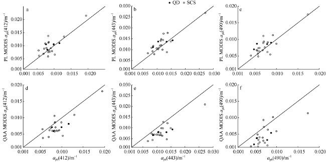
Fig.6 Scatter plots of match-ups between in situ and satellite-derived aph(λ) (λ=412, 443, 490) using the PL (a, b, c) and QAA (d, e, f) algorithms in the SCS and QD sea waters for MODIS-Aqua of relaxed match-ups (N=23). The solid line is 1︰1 line

图6 在宽松匹配法则下采用PL和QAA算法获得的南海开阔海域MODIS-Aqua aph(λ) (λ=412, 443, 490)产品值与相应实测值(N=23)之间的散点图
其中, a、b和c表示PL算法所得结果, d、e和f表示QAA算法所得结果, 图中直线为1︰1直线

Tab. 2 Statistics comparing in situ aph(λ) (λ=412, 443, 490) with MODIS-Aqua products basing on QAA and PL algorithms in the SCS and QD sea waters when relaxed match-ups are included

表2 在宽松的匹配法则下, 基于经验算法PL和半分析算法QAA反演获得的南海清洁海域(南海海区和琼东海区)MODIS aph(λ) (λ=412, 443, 490)产品值与实测值(N=23)的统计评价结果

QAA aph(412) QAA aph(443) QAA aph(490) PL aph(412) PL aph(443) PL aph(490)
APD/% 22.49 29.68 46.89 20.15 17.94 21.65
RPD/% -18.11 -29.33 -42.84 10.42 10.82 14.14
RMS 0.0023 0.0040 0.0039 0.0022 0.0024 0.0018
Ratio 0.7800 0.7099 0.5778 1.0543 1.0744 1.1448
SIQR 0.1139 0.0981 0.1706 0.1804 0.1507 0.1311
R2 0.6938 0.7231 0.3642 0.6178 0.7160 0.6682
Slope 0.8622 0.7434 0.6959 0.9210 0.8504 0.8312
Interception -0.0004 -0.0004 -0.0008 0.0015 0.0028 0.0020

注: APD为平均绝对误差, RPD为平均相对误差, RMS为均方根误差, Ratio为遥感产品值与实测值之比的中值, SIQR为遥感产品值与实测值之比的四分位, R2为决定系数, slope为斜率, Interception为截距。

2.2.2 基于不同的Chl-a产品反演算法, 采用PL算法的精度对比
根据赵文静等(2014)已有研究成果显示, 南海开阔海域多为低叶绿素浓度海域, 其浓度通常在0.25mg·m-3以下, 基于MODIS-Aqua Rrs(λ)产品采用区域优化后的OCI算法(赵文静, 2014)(简称NOCI算法)估算Chl-a精度更高。本文将南海NOCI 算法估算得到的Chl-a产品作为PL算法的输入, 进而估
算获得的aph(λ)(λ=412, 443, 490)结果见图7表3, 并与MODIS Chl-a标准业务化算法OC3获得的结果进行对比。结果发现, 基于南海区域优化后的NOCI算法获得的吸收系数产品精度远高于OC3 算法所获得的结果。就APD表现来看, 基于NOCI算法获得的aph(λ)(λ=412, 443, 490)较OC3算法提升近两倍, 特别是aph(490)最为突出, 且拟合的决定系数R2最高可达0.83。
上述结果表明, 对于南海清洁海区水体, 基于Lee算法反演获得的aph(λ)精度还有待进一步验证, 而经验算法PL可以获得相对较优的估算结果, 特别是采用区域优化后的Chl-a产品作为输入。
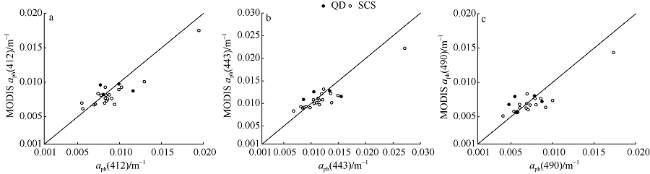
Fig. 7 Scatter plots of match-ups between in situ and satellite-derived aph(λ) (λ=412, 443, 490) using the PL algorithm based on regional algorithm NOCI-derived Chl-a in the SCS and QD sea waters for MODIS-Aqua of relaxed match-ups (N=23). The solid line is the 1︰1 line

图7 基于算法NOCI反演得到的Chl-a产品作为输入, 采用经验算法PL反演获得的MODIS-Aqua aph(λ)(λ=412, 443, 490)产品值与相应实测值(N=23)之间的散点图(图中实线为1:1直线)

Tab. 3 Statistics comparing in situ aph(412), aph(443) and aph(490) with MODIS-Aqua products using the PL algorithm, which is based on Chl-a products derived from the regional algorithm NOCI in the SCS and QD sea waters

表3 基于NOCI算法反演获得的Chl-a产品作为输入, 采用经验算法PL反演获得的南海海域和琼东海域MODIS aph(412), aph(443), aph(490)产品值与实测值(N=23)的统计评价结果

NOCI aph(412) NOCI aph(443) NOCI aph(490)
APD/% 12.14 11.87 13.89
RPD/% -4.02 -2.07 0.31
RMS 0.0014 0.0019 0.0014
Ratio 0.9331 0.9551 0.9842
SIQR 0.0859 0.0869 0.1024
R2 0.8012 0.8297 0.7538
Slope 0.7129 0.6250 0.6007
Interception 0.0020 0.0038 0.0026

注: APD为平均绝对误差, RPD为平均相对误差, RMS为均方根误差, Ratio为遥感产品值与实测值之比的中值, SIQR为遥感产品值与实测值之比的四分位, R2为决定系数, slope为斜率, Interception为截距。

3 结论

本文利用2003—2012年获取自南海海域、琼东海域、广东近岸海域和珠江口4个典型海区的固有光学参量aph(λ), 对比分析其光谱特征, 并初步探讨各海区浮游植物种群结构差异。结果表明, 以南海、琼东为代表的清洁海域和以广东沿岸、珠江口为代表的浑浊海域的表层aph(λ)光学特性具有明显的差异; aph(λ)在南海和琼东海域量值较小但在颗粒物系数中占据主导地位, 特别是对于443nm而言, 上述海区aph(443)占ap(443)的比例高达70%以上, 而在广东近岸与珠江口海域aph(λ)并不占优; 浮游植物单位吸收系数aph*(λ)系数存在明显的空间变化趋势, 表明浮游植物种群结构存在明显的区域特性, 色素组成和浓度变化以及色素打包效应均是造成其差异的可能原因。本文基于MODIS-Aqua Rrs(λ)产品对比分析了PL经验算法和QAA半分析算法在反演aph(λ) (λ=412, 443, 490)的精度。总体来说, 南海和琼东海域没有明显差别, 对于上述清洁海区, 经验算法PL精度更高, 遥感产品值相对于实测值而言有所高估, 412、443和490nm处的APD不超过22%, 且443nm处的浮游植物吸收系数精度最高, APD可达17.94%; 而基于QAA半分析算法所得的遥感产品值相对于实测值存在不同程度的低估; 若采用针对南海开阔海域所提出的优化算法NOCI获得的Chl-a作为输入, 基于PL算法获得的aph(λ) (λ=412, 443, 490)产品精度可以进一步提高, APD可提升近一倍, 量值介于11%~14%之间。因此, 本文通过南海各典型海区固有光学参量aph(λ)的现场光谱数据分析可知其具有明显的空间差异, 表明浮游植物结构种群也存在明显的区域特性, 对于采用MODIS-Aqua Rrs(λ)产品进行aph(λ)产品反演的精度来看, 基于水色遥感产品研究分析南海海区种群结构等具有较强的应用前景。
上述结果表明, 对于南海清洁海区水体, 基于Lee算法反演获得的aph(λ)精度还有待进一步验证, 而经验算法PL可以获得相对较优的估算结果, 特别是采用区域优化后的Chl-a产品作为输入。

The authors have declared that no competing interests exist.

[1]
曹文熙, 杨跃忠, 许晓强, 等, 2003. 珠江口悬浮颗粒物的吸收光谱及其区域模式[J]. 科学通报, 48(17): 1876-1882.

CAO WENXI, YANG YUEZHONG, XU XIAOQIANG, et al, 2003. Regional patterns of particulate spectral absorption in the Pearl River estuary[J]. Chinese Science Bulletin, 48(11): 2344-2351(in Chinese).

[2]
崔廷伟, 2006. 渤海生物光学特性与水色遥感反演[D]. 青岛:中国海洋大学.

CUI TINGWEI, 2006. Bio-optical properties and ocean color inversion of the Bohai Sea[D]. Qingdao: Ocean University of China (in Chinese).

[3]
郝艳玲, 曹文熙, 崔廷伟, 等, 2011. 基于半分析算法的赤潮水体固有光学性质反演[J]. 海洋学报, 33(1): 52-65.

HAO YANLING, CAO WENXI, CUI TINGWEI, et al, 2011. The retrieval of oceanic inherent optical properties based on semianalytical algorithm during the red ride[J]. Acta Oceanologica Sinica, 33(1): 52-65 (in Chinese).

[4]
王桂芬, 2008. 南海北部水体光学特性及水色反演模式[D]. 北京: 中国科学院大学.

WANG GUIFEN, 2008. Optical properties of seawater and ocean color models in Northern South China Sea[D]. Beijing: Chinese Academy of Sciences (in Chinese).

[5]
汪文琦, 董强, 商少凌, 等, 2009. 基于两种半分析算法的水体吸收系数反演[J]. 热带海洋学报, 28(5): 35-42.

WANG WENQI, DONG QIANG, SHANG SHAOLING, et al, 2009. An evaluation of two semi-analytical ocean color algorithms for waters of the South China Sea[J]. Journal of Tropical Oceanography, 28(5): 35-42 (in Chinese).

[6]
赵冬至, 罗虎, 傅云娜, 等, 2004. 海洋水色组分吸收系数的测定方法研究[J]. 海洋通报, 23(3): 81-86.

ZHAO DONGZHI, LUO HU, FU YUNNA, et al, 2004. Determination of spectral absorption coefficients of particles, dissolved material and phytoplankton for ocean discrete water samples[J]. Marine Science Bulletin, 23(3): 81-86 (in Chinese).

[7]
赵文静, 2014. 南海水色遥感产品精度检验及算法修正[D]. 北京: 中国科学院大学.

ZHAO WENJING, 2014. Assessment of ocean color products and modification of operational algorithms in the South China Sea[D]. Beijing: Chinese Academy of Sciences (in Chinese).

[8]
赵文静, 曹文熙, 王桂芬, 等, 2014. 南海海域MODIS-Aqua叶绿素浓度产品的精度对比和区域性算法修正[J]. 光学精密工程, 22(11): 3081-3090.

ZHAO WENJING, CAO WENXI, WANG GUIFEN, et al, 2014. Comparison of chlorophyll products derived from MODIS-Aqua and modification of operational algorithms in the South China Sea[J]. Optics and Precision Engineering, 22(11): 3081-3090 (in Chinese).

[9]
AIKEN J, FISHWICK J R, LAVENDER S, et al, 2007. Validation of MERIS reflectance and chlorophyll during the BENCAL cruise October 2002: preliminary validation of new demonstration products for phytoplankton functional types and photosynthetic parameters[J]. International Journal of Remote Sensing, 28(3-4): 497-516.

[10]
AIKEN J, HARDMAN-MOUNTFORD N J, BARLOW R, et al, 2008. Functional links between bioenergetics and bio-optical traits of phytoplankton taxonomic groups: an overarching hypothesis with applications for ocean colour remote sensing[J]. Journal of Plankton Research, 30(2): 165-181.

[11]
BAILEY S W, WERDELL P J, 2006. A multi-sensor approach for the on-orbit validation of ocean color satellite data products[J]. Remote Sensing of Environment, 102(1-2): 12-23.

[12]
BRICAUD A, MOREL A, BABIN M, et al, 1998. Variations of light absorption by suspended particles with chlorophyll a concentration in oceanic (case 1) waters: analysis and implications for bio‐optical models[J]. Journal of Geophysical Research: Oceans, 103(C13): 31033-31044.

[13]
CARDER K L, HAWES S, BAKER K A, et al, 1991. Reflectance model for quantifying chlorophyll a in the presence of productivity degradation products[J]. Journal of Geophysical Research: Oceans, 96(C11): 20599-20611.

[14]
CARDER K L, CHEN F R, LEE Z P, et al, 1999. Semianalytic moderate-resolution imaging spectrometer algorithms for chlorophyll a and absorption with bio-optical domains based on nitrate-depletion temperatures[J]. Journal of Geophysical Research: Oceans, 104(C3): 5403-5421.

[15]
CARDER K L, CHEN F R, CANNIZZARO J P, et al, 2004. Performance of the MODIS semi-analytical ocean color algorithm for chlorophyll-a[J]. Advances in Space Research, 33(7): 1152-1159.

[16]
CUI TINGWEI, ZHANG JIE, GROOM S, et al, 2010. Validation of MERIS ocean-color products in the Bohai Sea: a case study for turbid coastal waters[J]. Remote Sensing of Environment, 114(10): 2326-2336.

[17]
GORDON H R, BROWN O B, EVANS R H, et al, 1988. A semianalytic radiance model of ocean color[J]. Journal of Geophysical Research: Atmospheres, 93(D9): 10909-10924.

[18]
GORDON H R, WANG MENGHUA, 1994. Retrieval of water-leaving radiance and aerosol optical thickness over the oceans with SeaWiFS: a preliminary algorithm[J]. Applied Optics, 33(3): 443-452.

[19]
HU CHUANMIN, LEE Z, FRANZ B, 2012. Chlorophyll a algorithms for oligotrophic oceans: a novel approach based on three‐band reflectance difference[J]. Journal of Geophysical Research: Oceans, 117(C1): C01011.

[20]
LEE Z, WEIDEMANN A, KINDLE J, et al, 2007. Euphotic zone depth: its derivation and implication to ocean-color remote sensing[J]. Journal of Geophysical Research: Oceans, 112(C3): C03009.

[21]
LEE Z P, CARDER K L, MARRA J, et al, 1996. Estimating primary production at depth from remote sensing[J]. Applied Optics, 35(3): 463-74.

[22]
LEE Z P, CARDER K L, STEWARD R G, et al, 1998. An empirical algorithm for light absorption by ocean water based on color[J]. Journal of Geophysical Research: Oceans, 103(C12): 27967-27978.

[23]
LOISEL H, STRAMSKI D, 2000. Estimation of the inherent optical properties of natural waters from the irradiance attenuation coefficient and reflectance in the presence of Raman scattering[J]. Applied Optics, 39(18): 3001-3011.

[24]
LOISEL H, STRAMSKI D, MITCHELL B G, et al, 2001. Comparison of the ocean inherent optical properties obtained from measurements and inverse modeling[J]. Applied Optics, 40(15): 2384-2397.

[25]
O’REILLY J E, MARITORENA S, SIEGEL D A, et al, 2000. Ocean color chlorophyll a algorithms for SeaWiFS, OC2, and OC4: version 4[M]//HOOKER S B, FIRESTONE E R. SeaWiFS Postlaunch Calibration and Validation Analyses, Part 3. Greenbelt, Maryland: NASA Goddard Space Flight Center, 11: 9-23.

[26]
PARSONS T R, MAITA Y, LALLI C M, 1984. A manual of chemical and biological methods for seawater analysis[M]. Oxford: Pergamon Press: 173.

[27]
POPE R M, FRY E S, 1997. Absorption spectrum (380-700 nm) of pure water. II. Integrating cavity measurements[J]. Applied Optics, 36(33): 8710-8723.

[28]
PRIEUR L, SATHYENDRANATH S, 1981. An optical classification of coastal and oceanic waters based on the specific spectral absorption curves of phytoplankton pigments, dissolved organic matter, and other particulate materials[J]. Limnology and Oceanography, 26(4): 671-689.

[29]
QING SONG, ZHANG JIE, CUI TINGWEI, et al, 2012. Remote sensing retrieval of total absorption coefficient in the Bohai Sea[J]. Chinese Journal of Oceanology and Limnology, 30(5): 806-813.

[30]
ROESLER C S, PERRY M J, CARDER K L, 1989. Modeling in situ phytoplankton absorption from total absorption spectra in productive inland marine waters[J]. Limnology and Oceanography, 34(8): 1510-1523.

[31]
WANG MENGHUA, 2005. A refinement for the Rayleigh radiance computation with variation of the atmospheric pressure[J]. International Journal of Remote Sensing, 26(24): 5651-5663.

[32]
ZHAO W J, WANG G Q, CAO W X, et al, 2014. Assessment of SeaWiFS, MODIS, and MERIS ocean colour products in the South China Sea[J]. International Journal of Remote Sensing, 35(11-12): 4252-4274.

Outlines

/