
Journal of Tropical Oceanography >
An Argo trajectory simulation system for the South China Sea using Lagrangian method*
Received date: 2017-09-28
Request revised date: 2017-11-19
Online published: 2018-07-16
Supported by
National Natural Science Foundation of China (41525019, 41521005);“Global Changes and Air-Sea Interaction” of State Oceanic Administration (GASI-IPOVAI-02);Strategic Priority Research Program of the Chinese Academy of Sciences (XDA11010103)
Copyright
Our Argo trajectory simulation system for the South China Sea (SCS) contains the high-resolution ambient velocity field, a Lagrangian particle tracking model and the parameterization that represents the vertical motions of profiling Argo floats. This system is applied to simulate both conventional Argo floats (typically parked at 1000 m depth and profiling to 2000 m depth) and Deep Argo floats (parked at 500 m above the seafloor) within the SCS. By conducting the simulation with the counterparts of six core Argo floats serviced in the SCS, we find the displacements of synthetic floats from the simulation system resemble the real float displacements over 100-day time intervals. We therefore judge the simulations for core Argo are robust and further apply the system to simulate a potential Deep Argo array (with the resolution of 2°×2°×30 day). The results explore both the representativeness and the predictability of float displacements, which may provide a basis to understand float displacements in the deep layer as well as to contribute to planning deep Argo array program.
Key words: Argo; Lagrangian trajectory; the South China Sea
WANG Tianyu , DU Yan , XIA Yifan . An Argo trajectory simulation system for the South China Sea using Lagrangian method*[J]. Journal of Tropical Oceanography, 2018 , 37(4) : 9 -9 . DOI: 10.11978/2017105
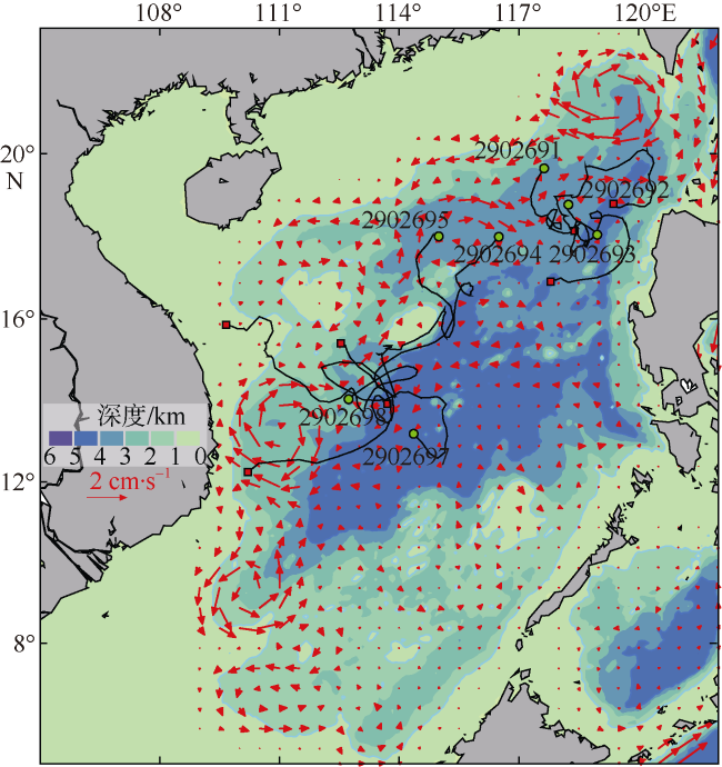
Fig. 1 Bottom topography of the South China Sea (shading), the annually-averaged velocity at 1000 m depth (red vector, units: cm•s-1) and the Argo trajectories (black lines). The release positions are indicated by green dots, and their end positions are, red rectangles图1 南海地形(填色)、2010年—2017年1000m层的平均流场(红色箭头, 单位: cm•s-1)与自动剖面浮标轨迹分布(黑色实线) |
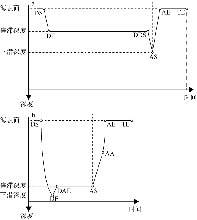
Fig. 2 Schematics of one float cycle for (a) conventional Argo floats and (b) Deep Argo floats during the test phase analyzed for this study. A conventional Argo cycle includes descent, parking, deep profiling, and surface telemetry. The schematic indicates the times when descent starts (DS), descent ends (DE), deep descent starts (DDS), ascent starts (AS), ascent ends (AE), and transmission ends (TE) (the definitions are based on Ollitrault et al, 2013). A Deep Argo cycle contains similar phases but with a slight change in the sequence, since the float first descends from DS to the ocean bottom (DE), and then rises to a parking pressure (DAE) for several days before rising to the surface, starting from AS. Ascent accelerates (at AA) at approximately 2000 m depth, and the float reaches the surface at AE图2 传统浮标(a)和新型深海浮标(b)完整工作周期示意图 |
Tab. 1 Information of core Argo floats trajectories表1 传统浮标轨迹信息 |
| 浮标序号 | 日期 | 经度/°E | 纬度/°N |
|---|---|---|---|
| 2902691 | 2016.9.6—2016.12.16 | 117°36′—117°54′ | 19°36′—18°12′ |
| 2902692 | 2016.9.7—2016.12.16 | 118°12′—118°00′ | 18°48′—18°54′ |
| 2902693 | 2016.9.8—2016.12.15 | 119°00′—118°42′ | 18°00′—18°18′ |
| 2902694 | 2016.9.9—2016.12.20 | 116°30′—115°42′ | 18°00′—16°54′ |
| 2902695 | 2016.9.12—2016.12.23 | 115°00′—115°12′ | 18°00′—16°12′ |
| 2902697 | 2016.9.15—2016.12.25 | 114°24′—112°42′ | 13°12′—14°12′ |
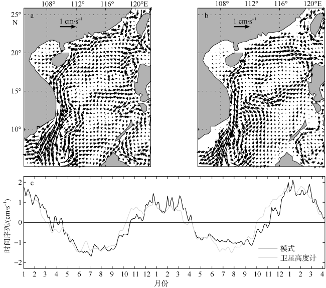
Fig. 3 The EOF mode-1 for ECCO2 50 m currents (a), TOPEX geostrophic currents (b) and Panel (c) denotes the PC-1 for ECCO2 (black curve) and TOPEX (gray curve)图3 ECCO2模式50m层流场(a)与高度计地转流场(b)经验正交分解第一模态空间分布和相对应的时间序列(c) |
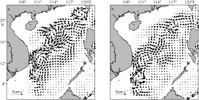
Fig. 4 The averaged velocity at mid-layer (1000 m) depth of the SCS: (a) winter and (b) summer. The release positions of synthetic floats are indicated by “+”. These location (Ⅰ: 16°12′N, 115°E; Ⅱ: 11°N, 110°30′E) are used in the following section图4 南海中层(1000m)环流分布 |
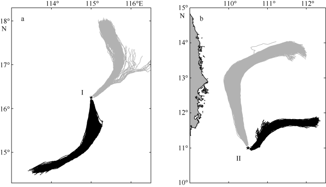
Fig. 5 Lagrangian motions of 100 synthetic conventional Argo floats in 100-day model simulations, which are released at (a) Ⅰ and (b) Ⅱ (shown in |
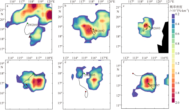
Fig. 6 PDFs of the simulated conventional Argo floats at the end of 100 days. Panels (a~f) correspond to the float series: 2902691, 2902692, 29026993, 2902694, 2902695, 2902697, and 2902698, which are listed in |
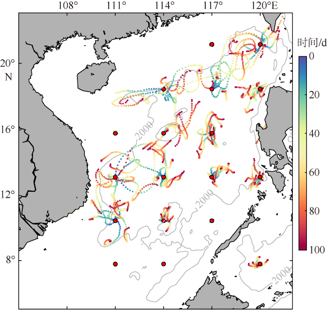
Fig. 7 The Lagrangian trajectories for a simulated deep Argos array. The resolution of the array is 2°×2°×30 day. The releasing positions of synthetic floats are marked by red dots. The trajectories are marked with colored dotted lines indicating the running time and overlapped by the 2000 m isobath that is marked by gray line图7 南海虚拟深海浮标阵列轨迹分布, 阵列分辨率为2°×2°×30d |
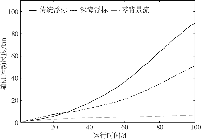
Fig. 8 The mean amplified random walk scales of synthetic floats as a function of run duration. The scale is calculated by the mean distance between each synthetic float and the center of mass of the ensemble of floats. The results of conventional Argo simulation are shown in black solid curve, and deep Argo simulation results are shown in dashed curve with the original random walk curve (without the ocean currents) indicated in gray图8 随机运动尺度随时间的增长曲线, 该尺度用每个浮标到浮标微团质量中心的平均距离来表征 |
The authors have declared that no competing interests exist.
| 1 |
|
| 2 |
|
| 3 |
|
| 4 |
|
| 5 |
|
| 6 |
|
| 7 |
|
| 8 |
|
| 9 |
|
| 10 |
|
| 11 |
|
| 12 |
|
| 13 |
|
| 14 |
|
| 15 |
|
| 16 |
|
| 17 |
|
| 18 |
|
| 19 |
|
| 20 |
|
| 21 |
|
| 22 |
|
| 23 |
|
| 24 |
|
| 25 |
|
| 26 |
|
| 27 |
|
/
| 〈 |
|
〉 |
