
Journal of Tropical Oceanography ›› 2023, Vol. 42 ›› Issue (6): 74-88.doi: 10.11978/2023032CSTR: 32234.14.2023032
• Marine Geophysics • Previous Articles Next Articles
Contrasting thermal states of the initial spreading systems between the Red Sea and the Gulf of California
XU Liuna1( ), LI Chunfeng1,2(), HUANG Liang1, ZHU Shuang1, YIN Yihong3
- 1. Department of Marine Science, Zhejiang University, Zhoushan 316021, China
2. Hainan Institute, Zhejiang University, Sanya 572025, China
3. Shandong Huakun Natural Resources Digital Industry Group, Jinan 250014, China
-
Received:2023-03-10Revised:2023-04-28Online:2023-11-10Published:2023-11-28 -
Supported by:National Natural Science Foundation of China(91858213); National Natural Science Foundation of China(42176055); Natural Science Foundation of Hainan Province, China(421CXTD441); Zhejiang University Cooperation Project with Zhoushan city(2019C81058)
Cite this article
XU Liuna, LI Chunfeng, HUANG Liang, ZHU Shuang, YIN Yihong. Contrasting thermal states of the initial spreading systems between the Red Sea and the Gulf of California[J].Journal of Tropical Oceanography, 2023, 42(6): 74-88.
share this article
Add to citation manager EndNote|Reference Manager|ProCite|BibTeX|RefWorks
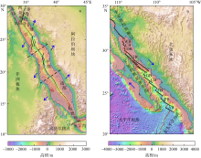
Fig. 1
Regional topographic map of the Red Sea (a) and regional topographic map of the Gulf of California (b). (a) The black dashed line indicates the segment boundaries of the Red Sea; red solid line indicates the Red Sea rift axis; solid black line indicates fault; blue arrows indicate directions of relative plate motion. (b) The red solid line indicates the spreading segment in the southern Gulf of California and the complex pull-apart basin in the northern Gulf of California; solid black line within the rift valley indicates transform fault; blue arrows indicate directions of relative plate motion. WB: Wagner Basin; CB: Consag Basin; DB: Delfin Basin; TB: Tiburon Basin; AB: Alarcon Basin; PB: Pescadero Basin; FB: Farallon Basin; CB: Carmen Basin; GB: Guaymas Basin. Bathymetric data are from GEBCO Compilation Group (2021). Fault data are from Styron et al (2020)"

Fig. 1
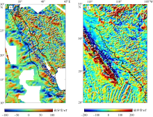
Fig. 2
Magnetic anomalies in the Red Sea (a) and the Gulf of California (b)"

Fig. 2
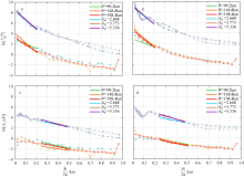
Fig. 3
Examples of radial averages of amplitude spectra of magnetic anomaly and their linear fits to calculating Z0 and Zt. (a) Calculating Z0 in the Red Sea; (b) calculating Z0 in the Gulf of California; (c) calculating Zt in the Red Sea; (d) calculating Zt in the Gulf of California. In each panel, the curves in the lower part are the results based on Fourier transform, while the curves in the upper part are the results based on wavelet transform"

Fig. 3
Tab. 1
Calculation window parameters for the Red Sea"
| 移动窗口大小/(km×km) | 移动窗口数量 | 移动步长/km |
|---|---|---|
| 99.2×99.2 | 55×67 | 49.6 |
| 148.8×148.8 | 36×44 | 74.4 |
| 198.4×198.4 | 27×33 | 99.2 |
Tab. 1
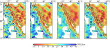
Fig. 4
Curie depth map of the Red Sea based on Fourier transform. (a) Window size = 99.2 km×99.2 km; (b) window size = 148.8 km×148.8 km; (c) window size = 198.4 km×198.4 km; (d) average Curie depth. The black dashed line delimits the Red Sea segment. The red solid line indicates the Red Sea rift axis. The solid black line indicates fault. The blue dashed line AA’ indicates the profile location of Fig. 8a"

Fig. 4
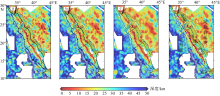
Fig. 5
Curie depth map of the Red Sea based on wavelet transform. (a) Central wavenumber |k0| =2.668; (b) central wavenumber |k0|=3.773; (c) central wavenumber |k0| =5.336; (d) average Curie depth"

Fig. 5
Tab. 2
Calculation window parameters for the Gulf of California"
| 移动窗口大小/(km×km) | 移动窗口数量 | 移动步长/km |
|---|---|---|
| 99.2×99.2 | 46×56 | 49.6 |
| 148.8×148.8 | 30×37 | 74.4 |
| 198.4×198.4 | 22×27 | 99.2 |
Tab. 2
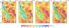
Fig. 6
Curie depth map of the Gulf of California based on Fourier transform. (a) Window size = 99.2 km×99.2 km; (b) window size = 148.8 km×148.8 km; (c) window size = 198.4 km×198.4 km; (d) average Curie depth. WB: Wagner Basin; CB: Consag Basin; DB: Delfin Basin; TB: Tiburon Basin; AB: Alarcon Basin; PB: Pescadero Basin; FB: Farallon Basin; CB: Carmen Basin; GB: Guaymas Basin. The solid red line indicates the spreading section in the southern Gulf of California and the complex pull-apart basin in the northern Gulf of California. The black solid line within the rift valley indicates transform fault. The pink dashed line BB’ indicates the profile location of Fig.8b"

Fig. 6
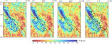
Fig.7
Curie depth map of the Gulf of California based on wavelet transform. (a) Central wavenumber |k0| =2.668; (b) central wavenumber |k0| =3.773; (c) central wavenumber |k0| =5.336; (d) average Curie depth"

Fig.7
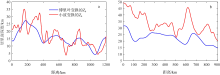
Fig. 8
Curie depth profiles. (a) Profile AA’ in the Red Sea region (Fig. 4d, 5d); (b) profile BB’ in the Gulf of California (Fig. 6d, 7d). Red line is the result based on the wavelet transform, and blue line is the result based on Fourier transform"

Fig. 8

Fig. 9
Distribution of the Curie depths. (a) Using Fourier transform; (b) using wavelet transform. The overlap between the two areas is shown in brown"
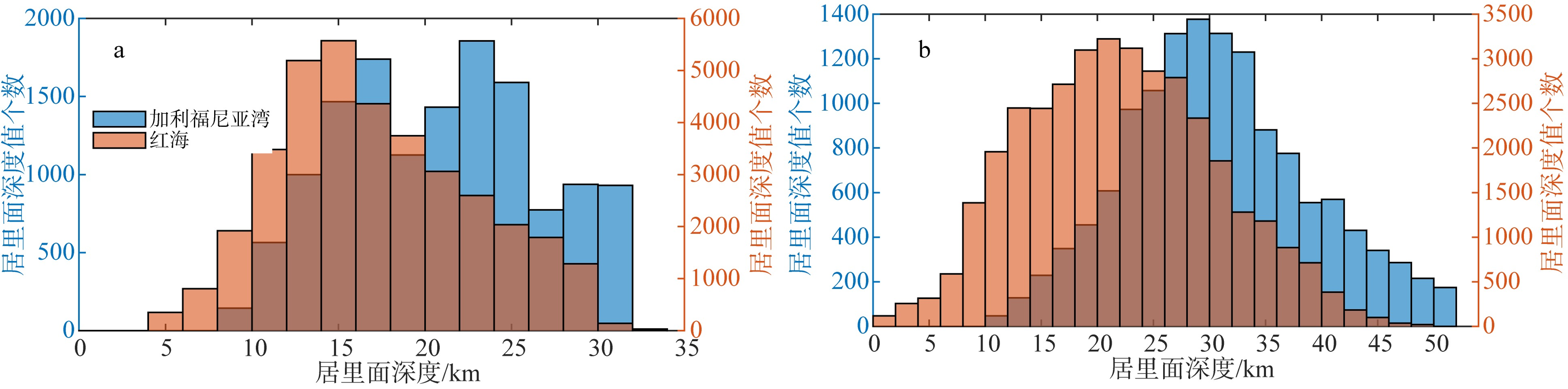
Fig. 9
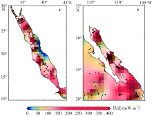
Fig. 10
Heat flow map of Red Sea (a) and Gulf of California (b). Data are gridded at a 0.5° interval. Black dots indicate the observation locations of heat flow data"

Fig. 10
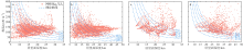
Fig. 11
Correlation between Curie depth and surface heat flow. (a) Results in the Red Sea based on Fourier transform; (b) results in the Red Sea based on Wavelet transform; (c) results in the Gulf of California based on Fourier transform; (d) results in the Gulf of California based on Wavelet transform. The blue dashed line shows the theoretical curves calculated based on the one-dimensional heat transfer model in Equation (10), where Tc = 550 °C, Ts = 5 °C, Zs = 4 km, hr = 5 km, and Hs = 1.37 μW·m-3 (Li et al, 2017), andκ is taken to vary from 1 to 6 W·(m℃) -1"

Fig. 11
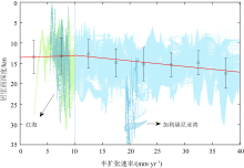
Fig. 12
Curie depths versus spreading rate around the spreading center (age of oceanic crust less than 5 Myr). The light green and light blue dots are the Curie depths within 5 Myr from the global reference Curie-point depth model GCDM (Li et al, 2017). The dark green and dark blue dots are the average Curie depths of the Red Sea and Gulf of California calculated in this study, respectively (sum of the results based on both Fourier and wavelet transform). The error bars are the standard deviation of the Curie depths of the light green and light blue dots at 5 mm·yr-1 intervals. The black squares in the error bars are the mean Curie depths"

Fig. 12
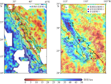
Fig. 13
Location of hydrothermal vents in the Red Sea (a) and the Gulf of California (b). ShD: Shaban Deep; KD: Kebrit Deep; ND: Nereus Deep; AD: Atlantis Ⅱ Deep; DD: Discovery Deep; SuD: Suakin Deep; RSR, 18°N: Red Sea Rift, 18°N; WB: Wagner Basin; CB: Consag Basin; Rv: Ringvent; GB: Guaymas Basin; PB: Pescadero Basin; AB: Alarcon Basin. The background shows the average Curie depth based on wavelet transform"

Fig. 13
| [1] |
宋珏琛, 李江海, 冯博, 2021. 慢速-超慢速扩张洋中脊热液活动及其机理[J]. 地质学报, 95(8): 2273-2283.
|
|
|
|
| [2] |
徐行, 姚永坚, 彭登, 等, 2018. 南海西南次海盆的地热流特征与分析[J]. 地球物理学报, 61(7): 2915-2925.
|
|
|
|
| [3] |
王淑杰, 翟世奎, 于增慧, 等, 2018. 关于现代海底热液活动系统模式的思考[J]. 地球科学, 43(3): 835-850.
|
|
|
|
| [4] |
doi: 10.3390/su15054549 |
| [5] |
doi: 10.1016/j.jseaes.2016.07.025 |
| [6] |
|
| [7] |
doi: 10.1016/j.proeps.2016.12.139 |
| [8] |
|
| [9] |
doi: 10.1016/j.epsl.2014.03.047 |
| [10] |
doi: 10.1016/j.geomorph.2016.08.028 |
| [11] |
|
| [12] |
doi: 10.1016/j.jvolgeores.2019.03.005 |
| [13] |
doi: 10.1016/j.sedgeo.2010.05.004 |
| [14] |
|
| [15] |
doi: 10.1016/j.apgeochem.2019.104467 |
| [16] |
|
| [17] |
doi: 10.1016/j.jsames.2020.102501 |
| [18] |
doi: 10.1016/0016-7037(96)00099-3 |
| [19] |
|
| [20] |
doi: 10.1029/2018JB016726 |
| [21] |
GEBCO COMPILATION GROUP, 2021. The GEBCO_2021 Grid-A continuous terrain model of the global oceans and land[DB/OL]. Published Data Library (PDL), [2023-03-09]. https://www.bodc.ac.uk/data/published_data_library/catalogue/10.5285/c6612cbe-50b3-0cff-e053-6c86abc09f8f/
|
| [22] |
doi: 10.5194/bg-15-5715-2018 |
| [23] |
doi: 10.1080/00206814.2014.941023 |
| [24] |
doi: 10.3390/en15228634 |
| [25] |
|
| [26] |
doi: 10.1016/j.tecto.2022.229604 |
| [27] |
doi: 10.1130/0016-7606(1972)83[3345:BMAAPT]2.0.CO;2 |
| [28] |
doi: 10.1130/0091-7613(1986)14<651:WAMMAS>2.0.CO;2 |
| [29] |
doi: 10.1016/j.jog.2010.08.003 |
| [30] |
|
| [31] |
doi: 10.1038/s41598-016-0028-x |
| [32] |
doi: 10.1111/j.1365-246X.2010.04702.x |
| [33] |
|
| [34] |
doi: 10.1002/ggge.v14.12 |
| [35] |
doi: 10.1007/s11600-019-00339-6 |
| [36] |
doi: 10.1016/0012-821X(85)90070-6 |
| [37] |
|
| [38] |
doi: 10.1029/2019GC008389 |
| [39] |
|
| [40] |
|
| [41] |
doi: 10.1016/j.epsl.2017.09.037 |
| [42] |
doi: 10.1190/1.1441926 |
| [43] |
|
| [44] |
|
| [45] |
doi: 10.1016/S0016-7037(00)00618-9 |
| [46] |
|
| [47] |
doi: 10.1016/j.isci.2020.101459 |
| [48] |
doi: 10.1016/j.marpetgeo.2021.105253 |
| [49] |
doi: 10.1007/s00024-012-0461-0 |
| [50] |
|
| [51] |
|
| [52] |
|
| [53] |
|
| [54] |
|
| [55] |
doi: 10.1038/205165a0 |
| [56] |
doi: 10.1016/S0040-1951(99)00072-4 |
| [57] |
doi: 10.1038/s41598-019-50200-5 |
| [58] |
|
| [59] |
doi: 10.1016/j.chemgeo.2015.04.001 |
| [60] |
|
| [61] |
doi: 10.1130/GES02082.1 |
| [62] |
doi: 10.1016/S0012-821X(02)01081-6 |
| [63] |
doi: 10.1016/j.tecto.2014.11.002 |
| [64] |
doi: 10.1016/j.gr.2022.09.010 |
| [65] |
doi: 10.1093/gji/ggab257 |
| [66] |
doi: 10.1007/s11001-020-09401-1 |
| [1] | REN Ziqiang, SHI Xiaobin, WANG Xiaofang, ZHAO Peng, SHEN Yongqiang. Deep thermal state in the Nansha Trough of South China Sea and its tectonic implications [J]. Journal of Tropical Oceanography, 2021, 40(4): 98-109. |
| [2] | XU Ziying, YANG Xiaoqiu, SHI Xiaobin, ZENG Xin, ZHAO Junfeng, YU Chuanhai. Effects on the results of seafloor heat flow measurements by probe tilt [J]. Journal of Tropical Oceanography, 2016, 35(4): 95-101. |
| [3] | MA Hui, XU He-hua, ZHAO Jun-feng, WAN Ju-ying, CHEN Ai-hua, LIU Tang-wei. Thermal structure of Nansha Trough Foreland Basin [J]. Journal of Tropical Oceanography, 2012, 31(3): 155-161. |
| [4] | FENG Xiang-bo,YAN Yi-xin. Coastal sea-state monitoring system off Taiwan Island: Its establishment and data analysis [J]. Journal of Tropical Oceanography, 2011, 30(1): 35-42. |
|
||