
Journal of Tropical Oceanography ›› 2026, Vol. 45 ›› Issue (1): 154-167.doi: 10.11978/2025218CSTR: 32234.14.2025218
Previous Articles Next Articles
Analysis of the mechanisms underlying the low-frequency variability of the low-salinity tongue in the southeastern Indian Ocean*
PANG Yanran1,2( ), SUN Qiwei3,4, ZHANG Yuhong1,2,5, ZHANG Ying1,2,5, CHI Jianwei1,2,5, DU Yan1,2,5()
- 1State Key Laboratory of Tropical Oceanography, South China Sea Institute of Oceanology, Chinese Academy of Sciences, Guangzhou 511458, China
2University of Chinese Academy of Sciences, Beijing 100049, China
3Southern Marine Science and Engineering Guangdong Laboratory (Guangzhou), Guangzhou 511458, China
4Department of Ocean Science and Hong Kong Branch of the Southern Marine Science and Engineering Guangdong Laboratory (Guangzhou), Hong Kong University of Science and Technology, Hong Kong 999077, China
5Guangdong Key Lab of Ocean Remote Sensing and Big Data (LORS), South China Sea Institute of Oceanology, South China Sea Institute of Oceanology, Chinese Academy of Sciences, Guangzhou 510301, China
-
Received:2025-11-17Revised:2025-11-25Online:2026-01-10Published:2026-01-30 -
Contact:Du Yan. email:duyan@scsio.ac.cn -
Supported by:National Natural Science Foundation of China(42090042); National Natural Science Foundation of China(42306026); Chinese Academy of Sciences(183311KYSB20200015); South China Sea Institute of Oceanology(LTO2306); South China Sea Institute of Oceanology(SCSIO202201); South China Sea Institute of Oceanology(SCSIO2023HC07); Key Talents Project of Guangdong Province(2024TQ08A880)
CLC Number:
- P732.6
Cite this article
PANG Yanran, SUN Qiwei, ZHANG Yuhong, ZHANG Ying, CHI Jianwei, DU Yan. Analysis of the mechanisms underlying the low-frequency variability of the low-salinity tongue in the southeastern Indian Ocean*[J].Journal of Tropical Oceanography, 2026, 45(1): 154-167.
share this article
Add to citation manager EndNote|Reference Manager|ProCite|BibTeX|RefWorks
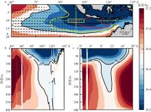
Fig. 1
Three-dimensional structure of the low-salinity water tongue in the southeastern Indian Ocean. (a) Climatological distribution of sea surface salinity (color shading, units: ‰) and surface currents (vectors, units: m·s−1), overlaid by the 34.6 ‰ isohaline at 0 m (black line), 50 m (yellow line), and 100 m (red line). The green lines indicate the transect location in panels (b) and (c), respectively, and the green box corresponds to the averaging area in Fig 2c; (b) climatological distribution of salinity (color shading, units: ‰) along the 10°S meridional section; (c) similar to (b), but for the 100°E zonal section"

Fig. 1

Fig. 2
Interannual-decadal variations in the three-dimensional structure of the low-salinity tongue in the southeastern Indian Ocean. (a) Longitude-time Hovmöller diagram of sea surface salinity (shaded, units: ‰) averaged over 9° to 11°S, with the 34.6 ‰ isohaline at 0 m (black line), 50 m (yellow line), and 100 m (red line) after 13-month running mean; (b) similar to (a), but for the latitude-time Hovmöller diagram of salinity averaged over 97° to 102°E; (c) depth-time diagram of salinity (shaded, units: ‰) averaged within 95° to 105°E and 9° to 11°S, with the 34.6 ‰ isohaline at 0 m (black line) after a 13-month running mean"
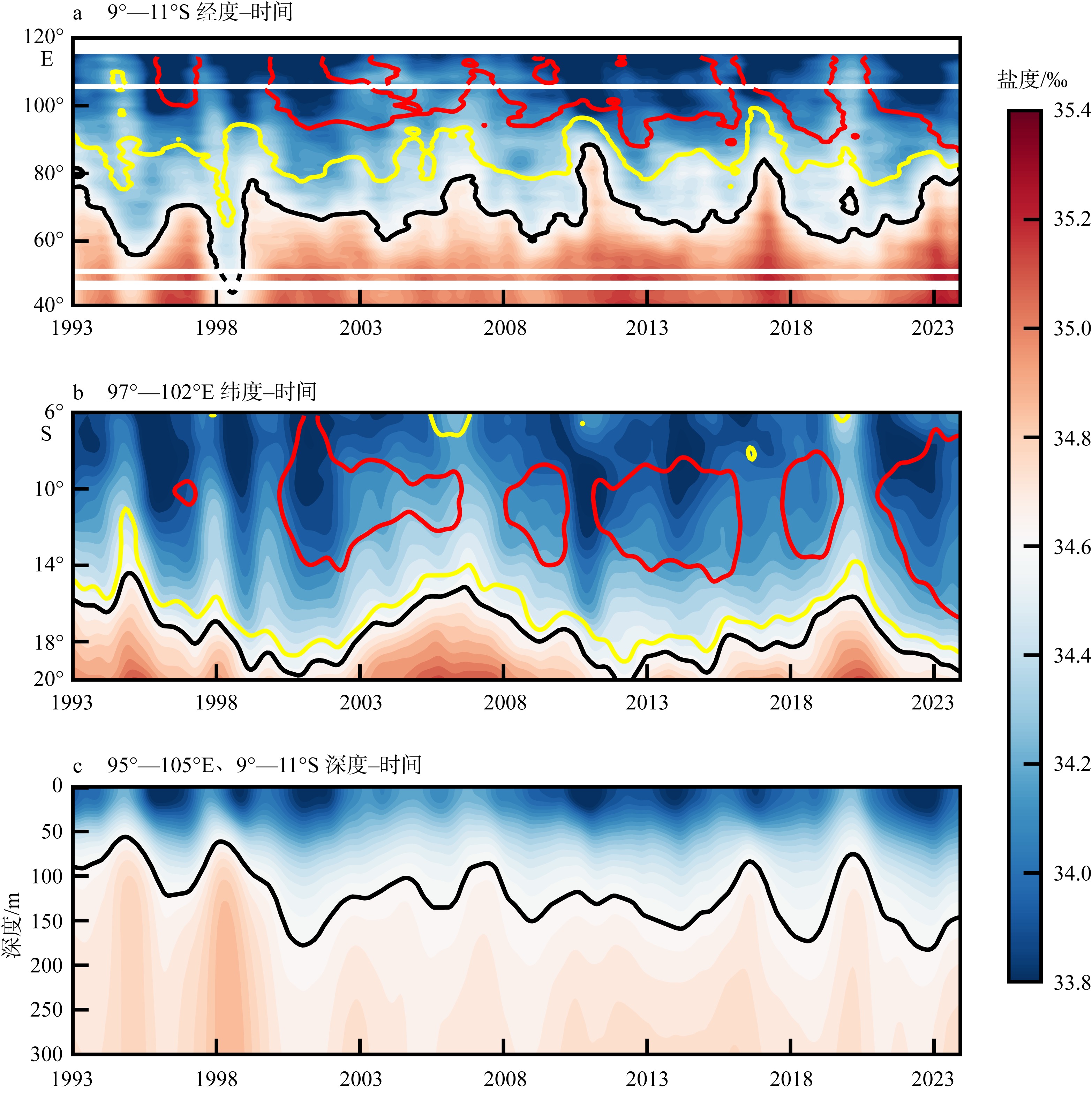
Fig. 2
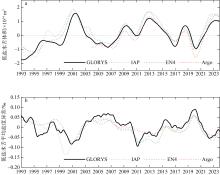
Fig. 3
Time series of the volume and average salinity anomalies of the low-salinity tongue from multi-source data (water bounded by the 34.6 ‰ isohaline within the upper 200 m in the region 4° to 20°S, 40° to 145°E. (a) Time series of the volume of the low-salinity tongue in the upper 200 m, derived from the GLORYS12V1 (black line), IAP (blue dashed line), EN4 (green dashed line), and Argo (red dashed line) datasets; (b) similar to (a), but for the average salinity anomalies of the low-salinity tongue"

Fig. 3
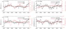
Fig. 4
Relationship between the volume and salinity of low salinity tongue in the surface (0 to 50 m) and subsurface (50 to 200 m) layers and local precipitation and ITF salt flux. (a) Time series of the volume of the low-salinity tongue at 0 to 50 m and local precipitation; local precipitation refers to the rainfall over areas surrounded by the low-salinity water; (b) time series of the volume of the low-salinity tongue at 50 to 200 m and the salinity flux through section IX1; (c) time series of the average salinity anomalies of the low-salinity tongue at 0 to 50 m and local precipitation; (d) time series of the average salinity anomalies of the low-salinity tongue at 50 to 200 m and the salinity flux through section IX1. The solid red line and dashed red line represent the 7-year running mean and 13-month running mean, respectively"
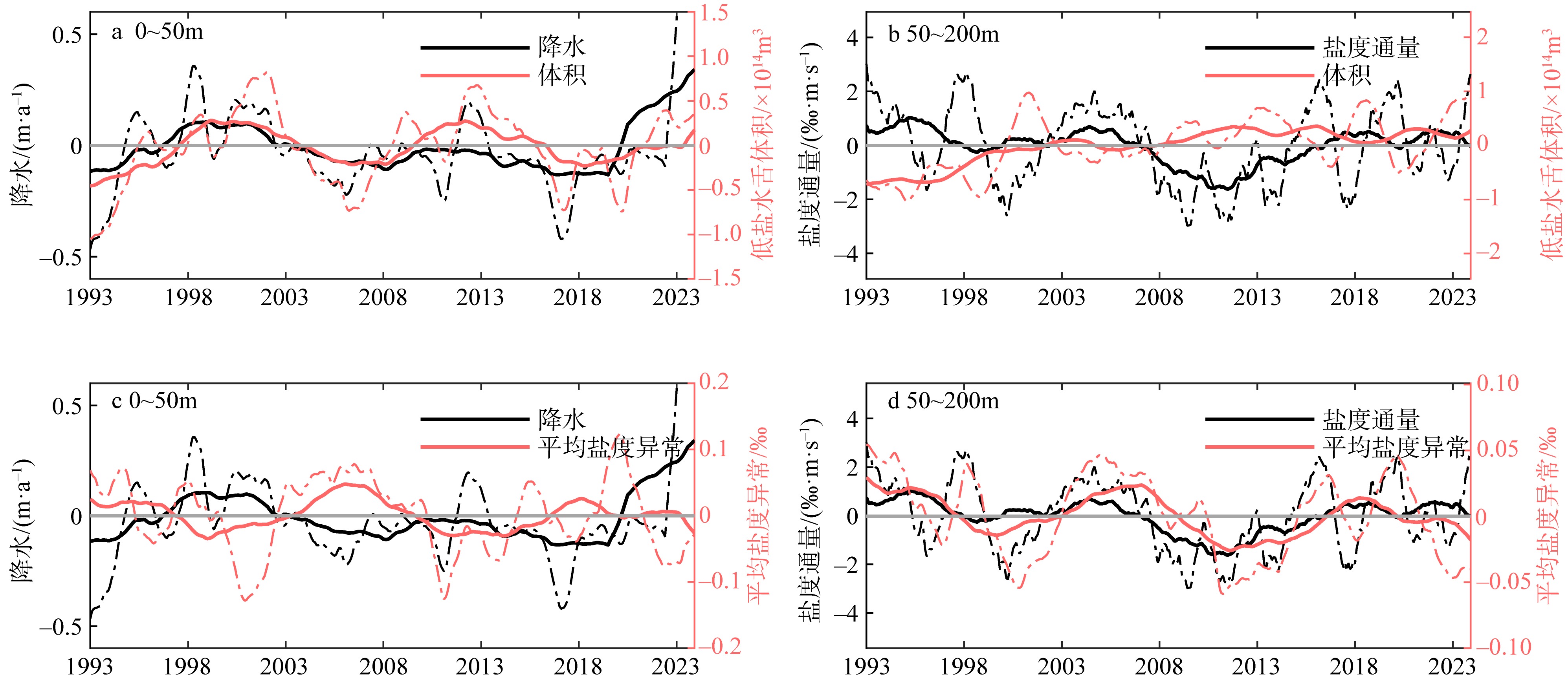
Fig. 4
Fig. 5
Spectral characteristics of the low-salinity tongue, local precipitation, and ITF salt flux, and the salinity-velocity structure across section IX1. (a) Time series of the salt flux through section IX1 (solid black line: 7-year running mean; dashed black line: 13-month running mean) and the mean current velocity (red line) across the section; (b) power spectrum of the volume (black line) and average salinity anomalies (blue line) of the low-salinity tongue with the red line denoting the red-noise spectrum; (c) similar to (b), but for the salt flux through section IX1 (black line) and local precipitation (blue line); (d), (e) similar to (a), but based on EN4 salinity data (1970 to 2023) and IAP salinity data (1960 to 2023)"
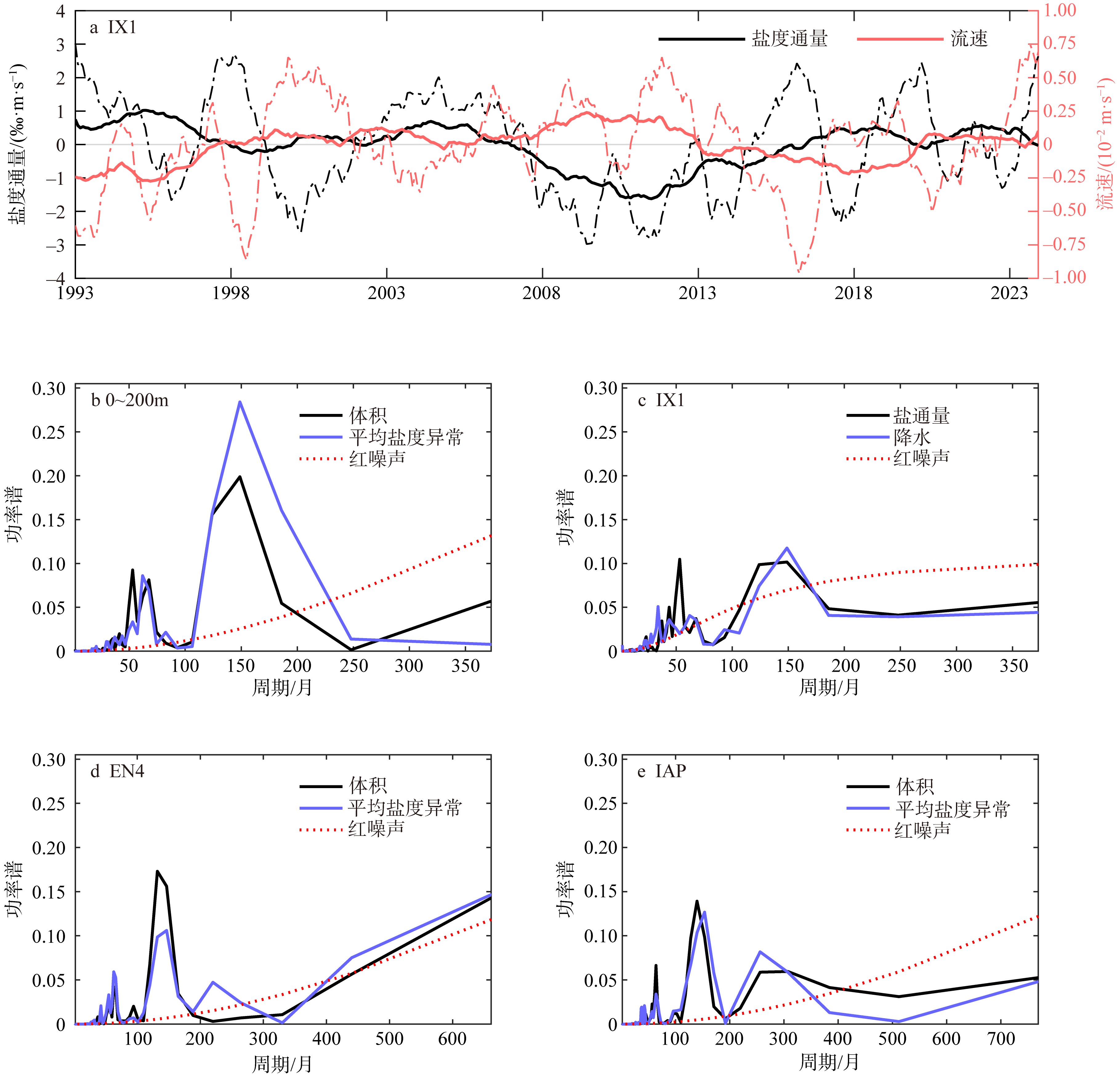
Fig. 5
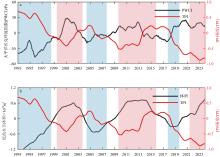
Fig. 6
Time series of PWCI, TPI, and the volume of the low-salinity tongue. (a) The TPI (red line) and PWCI (black line) after a 7-year running mean; red shading denotes periods when the volume of the low-salinity tongue is greater than 0.3σ (freshing periods), and blue shading denotes periods when it is less than −0.3σ (salinification periods); (b) similar to (a), but for TPI (red line) and the volume of the low-salinity tongue in the upper 200 m (black line)"

Fig. 6
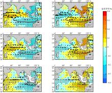
Fig. 7
Ocean salinity and current anomalies in the upper 100 m during freshening and salinification periods. (a) Composite map at the depth of 0 m during the freshening periods (defined as periods when the index of the low-salinity tongue volume is below −0.3σ), showing current vectors (units: cm·s−1), salinity anomalies (color shading, units: ‰), the climatological 34.6 ‰ isohaline (green line), and the contemporary 34.6 ‰ isohaline (purple line); (c, e): similar to (a), but for the depths of 50 m and 100 m, respectively; (b) similar to (a), but for the salinification periods (defined as periods when the index of the low-salinity tongue volume is greater than 0.3σ); (d, f) similar to (b), but for the depth of 50 m and 100 m, respectively; black dots indicate areas that are statistically significant at the 95 % confidence level"

Fig. 7
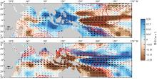
Fig. 8
Variations in Indo-Pacific wind, SLP, and precipitation during the freshening and salinification periods. (a) Composite anomalies of wind fields (vectors, units: m·s−1), sea level pressure (contours, units: Pa), and precipitation (color shading, units: m·a−1) over the 20 months preceding the freshening periods (defined as periods when the index of the low-salinity tongue volume is less than −0.3σ), with black dots indicating areas that are statistically significant at the 95 % confidence level; (b) similar to (a), but for the 20 months preceding the salinification periods (defined as periods when the index of the low-salinity tongue volume is greater than 0.3σ)"

Fig. 8
| [1] |
|
| [2] |
doi: 10.1175/1520-0493(1969)097<0163:ATFTEP>2.3.CO;2 |
| [3] |
|
| [4] |
doi: 10.1175/JCLI-D-20-0366.1 |
| [5] |
doi: 10.1038/srep16050 pmid: 26522168 |
| [6] |
doi: 10.5670/oceanog |
| [7] |
doi: 10.1175/2010JCLI3377.1 |
| [8] |
doi: 10.1126/science.1212222 pmid: 22539717 |
| [9] |
doi: 10.1002/2015GL065848 |
| [10] |
doi: 10.1186/s40562-018-0102-2 |
| [11] |
|
| [12] |
doi: 10.1002/jgrc.v118.12 |
| [13] |
doi: 10.1038/379146a0 |
| [14] |
doi: 10.1029/97GL01061 |
| [15] |
doi: 10.1038/nature02038 |
| [16] |
doi: 10.1175/2009JCLI2981.1 |
| [17] |
doi: 10.5194/gmd-9-3993-2016 |
| [18] |
doi: 10.1175/JPO-D-22-0205.1 |
| [19] |
|
| [20] |
doi: 10.1007/s00382-015-2525-1 |
| [21] |
|
| [22] |
|
| [23] |
doi: 10.1002/jgrc.v121.4 |
| [24] |
doi: 10.1002/grl.v44.3 |
| [25] |
doi: 10.1175/JCLI-D-19-0056.1 |
| [26] |
|
| [27] |
doi: 10.1007/s00382-019-04795-0 |
| [28] |
|
| [29] |
|
| [30] |
doi: 10.1175/1520-0485(2002)032<1404:EOTITO>2.0.CO;2 |
| [31] |
doi: 10.5194/os-14-1093-2018 |
| [32] |
|
| [33] |
doi: 10.3389/fmars.2022.1097634 |
| [34] |
|
| [35] |
doi: 10.1002/jgrc.v120.12 |
| [36] |
doi: 10.1175/JCLI-D-23-0248.1 |
| [37] |
doi: 10.1038/s41558-024-02033-y |
| [38] |
doi: 10.1175/JCLI-D-21-0288.1 |
| [39] |
doi: 10.1175/JCLI-D-23-0725.1 |
| [40] |
doi: 10.1002/grl.v40.21 |
| [41] |
doi: 10.3389/fmars.2023.1181278 |
| [42] |
doi: 10.1029/2018JC014574 |
| [43] |
doi: 10.1175/JCLI-D-21-0485.1 |
| [44] |
doi: 10.1016/j.dynatmoce.2010.02.003 |
| [45] |
|
| [46] |
doi: 10.1175/1520-0442(1998)011<0676:TITATG>2.0.CO;2 |
| [47] |
|
| [48] |
|
| [49] |
doi: 10.1002/jgrc.v119.2 |
| [50] |
doi: 10.1175/JCLI-D-20-0331.1 |
| [51] |
doi: 10.1038/s41467-021-26693-y pmid: 34764254 |
| [52] |
doi: 10.1175/JCLI-D-21-0122.1 |
| [53] |
doi: 10.1002/jgrc.v121.7 |
| [54] |
doi: 10.1007/s00382-022-06231-2 |
| [55] |
doi: 10.1002/jgrc.20392 |
| [56] |
doi: 10.1007/s00382-016-2984-z |
| [57] |
doi: 10.1175/JCLI-D-17-0271.1 |
| [58] |
|
| [59] |
doi: 10.1007/s00343-023-3129-y |
| [60] |
|
| [1] | LIN Guihuan, YAN Youfang, LIU Ying. Ocean stratification in the Indonesian-Australian basin and its influencing factors [J]. Journal of Tropical Oceanography, 2024, 43(4): 57-67. |
| [2] | QI Peng, LI Shasha, CAO Lei. Local factors affecting decadal variability of Luzon Strait transport [J]. Journal of Tropical Oceanography, 2016, 35(4): 1-10. |
| [3] | YANG Yali, DU Yan. Decadal variability of oceanic advection in the South China Sea associated with ENSO and Indian-Ocean Basin and its impacts on SST [J]. Journal of Tropical Oceanography, 2016, 35(1): 72-81. |
| [4] | ZENG Zhi, CHEN Xue-en, TANG Sheng-quan, WANG Wei-dong, GAO Rong-lu, YUAN Nan. Evaluation of SMOS sea surface salinity data in the equatorial Pacific and its correction using neural network [J]. Journal of Tropical Oceanography, 2015, 34(6): 35-41. |
| [5] | WANG Jian, DU Yan, ZHENG Shao-jun, LIU Kai. Interannual variability of Indonesian throughflow in the Makassar Strait during 2004~2011 [J]. Journal of Tropical Oceanography, 2014, 33(6): 9-16. |
| [6] | LIU Kai,SUN Zhao-bo,DU Yan. Power spectrum analysis of Indonesian Throughflow based on INSTANT data [J]. Journal of Tropical Oceanography, 2011, 30(6): 1-9. |
| [7] | LIU Qin-yan,ZHOU Wen. Relationship between typhoon activity in the northwestern Pacific and the up-per-ocean heat content on interdecadal time scale [J]. Journal of Tropical Oceanography, 2010, 29(6): 8-14. |
| [8] | LIU Xiang-cui,LIU Hai-long,LI Wei,LIN Peng-fei. Geostrophic transport of the Indonesian Throughflow estimated by using the Argo data [J]. Journal of Tropical Oceanography, 2009, 28(5): 75-82. |
|
||