
Journal of Tropical Oceanography >
A case study of the influence of the cold surge and ocean front on the evolution of atmospheric ducts in the northwestern South China Sea
Copy editor: YIN Bo
Received date: 2021-12-31
Revised date: 2022-03-12
Online published: 2022-03-21
Supported by
Key Special Project for Introduced Talents Team of Southern Marine Science and Engineering Guangdong Laboratory (Guangzhou)(GML2019ZD0304)
National Natural Science Foundation of China(41676018)
Science and Technology Planning Project of Guangzhou City, China(202002030490)
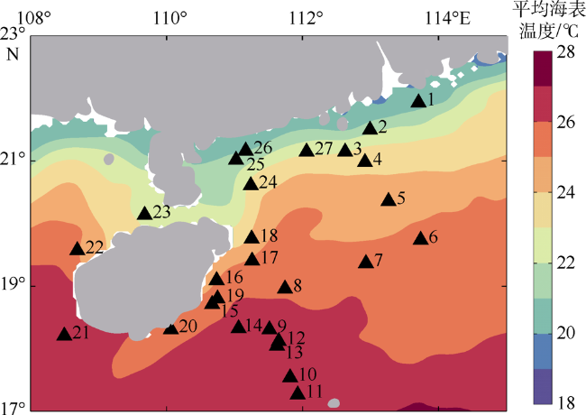
Using the GPS sonde data collected at the northwestern part of the South China Sea in the winter of 2012, we studied the influences of cold surge and ocean front on the characteristics of the atmospheric duct. In the investigation period, the main atmospheric ducts were elevated ducts, with an average bottom height of 738.64 m, an average thickness about 185.17 m, and an average strength of 10.21 M-unit. In the early stage of investigation, the weather was stable, and the northeast monsoon was weak in the study area, and the elevated ducts on the warm side of the front were relatively deep and strong but not very high. The main reason for the elevated duct layer is the temperature inversion layer on top of the atmospheric boundary layer from 925 hPa to 850 hPa, which also has significant diurnal characteristics. In the middle of the investigation, a cold surge significantly strengthened the northeast monsoon which destroyed the inversion layer at the top of the atmospheric boundary layer. As a result, the height of the elevated ducts rises significantly, and the duct layer becomes thinner and weaker. Meanwhile, the disturbance of the negative atmospheric modified refractive index gradient was weak due to the depressed turbulence over the cold side of the front. Thus, forming a stable and robust duct layer is difficult, and there is no significant diurnal variation. However, when the warm and humid air flows southwesterly covering the cold side of the front, it is highly possible to form a stable surface duct.
SHI Rui , CHEN Ju , HE Yunkai , SUI Dandan , SHU Yeqiang . A case study of the influence of the cold surge and ocean front on the evolution of atmospheric ducts in the northwestern South China Sea[J]. Journal of Tropical Oceanography, 2022 , 41(5) : 29 -42 . DOI: 10.11978/2021190
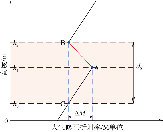
图2 大气波导特征参数示意图。图中h0表示波导层底高度, h1表示陷获层高度, h2表示波导层顶高度; d0表示波导层厚度, ΔM表示波导层强度。A、B、C点分别为大气修正折射率梯度转为负值高度、大气修正折射率梯度转为正值高度和A点下方观测到与B点相同折射率的高度。粉色区域表示大气波导层 Fig. 2 Schematic diagram of the basic parameters to describe the characteristics of atmospheric duct. The pink layer is the duct layer, where h0 is the bottom heigh of the duct layer, h1 is the height of trapping layer, and h2 is top height of the duct layer. d0 and ΔM respectively denotes the depth and strength of the duct. A point marks the place where the gradient of M turns into negative, B point marks the place where the gradient of M turns into positive, and C point marks the place where have the same value of M as B point |
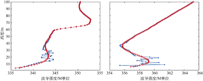
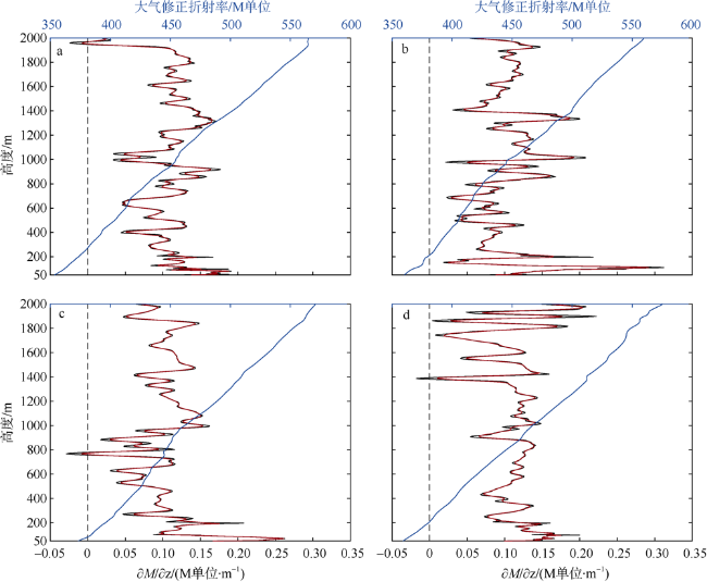
图3 根据公式(3)计算的航次期间原始大气修正折射率M (蓝线)及多项式拟合和滑动平均后的大气修正折射率M廓线(红线), 以2号(a)和17号(b)探空结果为例Fig. 3 Vertical profile of the atmospheric modified refractive index M before (blue lines) and after polynomial fitting and moving average (red lines), the results of sounding No. 2 (a) and No. 17 (b) are shown as examples here |
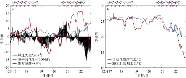
图4 12月17日至22日船载气象观测站记录风速矢量、海平面气压与相对湿度(a)和海面气温和SBE-21走航温盐计观测水温(b)图a中纵坐标为风矢量绝对值大小, 0值线为风矢量尾部。横坐标轴红色倒三角表示探空释放点及编号变量值表示经同图处理后的各变量的大小 Fig. 4 (a) The wind speed vector, sea level pressure, and relative humidity observed by the shipboard automatic weather station (AWS) from December 17th to 22nd; (b) The sea surface air temperature from AWS and the water temperature recorded by the SBE-21 sailing thermometer and salinometer installed on the bottom of the ship. The ordinate in |
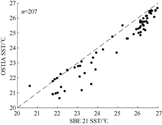
图5 12月16日至22日SBE 21船用走航温盐计观测海温与OSTIA数据产品平均海表温度(SST)对比n为样本数, 为当日与研究区域内OSTIA格点最接近的SBE 21观测记录总数。虚线表示斜率为1的线性回归拟合曲线 Fig. 5 Comparison of the water temperature recorded by the SBE 21 from December 16th to 22nd and the OSTIA SST. n is the number of samples, which is the sum of the number of SBE 21 observation records closest to the OSTIA grid point in the study area on that day. Dashed line is the linear regression line with a slope of one |
表1 2012年12月13日至22日南海北部航次GPS探空观测时间、海表温度及是否观测到波导现象记录Tab.1 Information for the northern South China Sea investigation observation from December 13rd to 22nd, 2012, including the GPS sounding observation time, sea surface temperature, and whether the atmospheric ducts were observed |
| 探空编号 | 观测时间 | 海表温度/℃ | 表面/蒸发波导 | 悬空波导 |
|---|---|---|---|---|
| 1 | 13日09时 | 20.45 | √ | |
| 2 | 13日14时 | 21.63 | √ | √ |
| 3 | 13日20时 | 23.02 | ||
| 4 | 14日14时 | 23.71 | √ | |
| 5 | 14日20时 | 24.67 | √ | √ |
| 6 | 15日02时 | 25.57 | √ | |
| 7 | 15日08时 | 25.93 | √ | √ |
| 8 | 15日14时 | 26.35 | √ | √ |
| 9 | 15日20时 | 26.76 | √ | |
| 10 | 16日02时 | 26.66 | √ | |
| 11 | 16日08时 | 26.89 | √ | √ |
| 12 | 16日14时 | 26.47 | √ | √ |
| 13 | 16日20时 | 26.48 | √ | |
| 14 | 17日02时 | 26.38(26.49) | √ | |
| 15 | 17日08时 | 25.71(25.91) | √ | √ |
| 16 | 17日14时 | 25.25(25.74) | √ | |
| 17 | 17日20时 | 25.27(25.81) | √ | |
| 18 | 18日02时 | 24.19(24.99) | √ | √ |
| 19 | 18日11时 | 25.56(25.93) | √ | √ |
| 20 | 18日14时 | 25.49(25.76) | √ | |
| 21 | 20日20时 | 26.67(26.82) | √ | |
| 22 | 21日02时 | 24.97(25.15) | √ | |
| 23 | 21日08时 | 22.65(22.77) | √ | |
| 24 | 21日14时 | 23.14(23.49) | √ | |
| 25 | 21日17时 | 21.23(21.79) | ||
| 26 | 21日20时 | 20.92(21.32) | √ | |
| 27 | 22日01时 | 22.13(22.73) | √ | |
| 合计次数(发生概率) | 17(0.62) | 17(0.62) |
注: 括号外数字为OSTIA水温值, 括号内数字为OSTIA数据与SBE 21观测水温的平均海表温度值。表中统计波导判别条件为ΔM >1M单位。√表示该时刻观测到波导现象, 空白表示该时刻未观测到波导现象 |
表2 航次期间观测到50m以下表面波导的具体参数(仅统计ΔM >1M单位的波导层)Tab. 2 Characteristics of the surface duct observed during the investigation, and only the atmospheric duct layer with ΔM > 1 M-unit was counted |
| 探空编号 | 观测时间 | 海表温度/℃ | 波底高度/m | 波导厚度/m | 波导强度/M单位 | ||
|---|---|---|---|---|---|---|---|
| 5 | 14日20时 | 24.67 | 28.0 | 17.0* | 2.55 | ||
| 7 | 15日08时 | 25.93 | 23.0 | 12.0* | 3.22 | ||
| 7 | 15日08时 | 25.93 | 44.0 | 22.0 | 2.67 | ||
| 8 | 15日14时 | 26.35 | 23.0 | 15.0* | 12.7 | ||
| 11 | 16日08时 | 26.89 | 23.0 | 23.0* | 2.53 | ||
| 12 | 16日14时 | 26.47 | 25.0 | 23.0* | 4.92 | ||
| 15 | 17日08时 | 25.91 | 28.0 | 30.0* | 4.61 | ||
| 16 | 17日14时 | 25.74 | 29.0 | 29.0* | 7.48 | ||
| 17 | 17日20时 | 25.81 | 26.0 | 18.0* | 3.37 | ||
| 18 | 18日02时 | 24.99 | 26.0 | 18.0* | 1.35 | ||
| 19 | 18日11时 | 25.93 | 23.0 | 17.0 | 2.04 | ||
| 22 | 21日02时 | 25.15 | 35.0 | 10.0* | 4.32 | ||
| 23 | 21日08时 | 22.77 | 13.5 | 22.0 | 5.08 | ||
| 24 | 21日13时 | 23.49 | 39.0 | 21.0 | 5.20 | ||
| 26 | 21日20时 | 21.32 | 7.5 | 18.0 | 3.03 | ||
| 27 | 22日01时 | 22.13 | 23.0 | 26.0 | 1.25 | ||
| 平均值 | 26.0 | >20.06 | 4.15 | ||||
注: *表示未能确定波导层底部高度, 而是从观测开始高度估计的波导厚度 |
表3 航次期间观测到波底高度在50m以上悬空波导的具体参数(仅统计ΔM >1M单位的波导层)Tab. 3 Characteristics of the elevated ducts observed during the investigation, and only the waveguide layer with ΔM > 1 M-unit was counted |
| 探空编号 | 观测时间 | 海表温度/℃ | 波底高度/m | 波导厚度/m | 波导强度/M单位 |
|---|---|---|---|---|---|
| 1 | 13日09时 | 20.45 | 1608.70 | 76.30 | 4.06 |
| 2 | 13日14时 | 21.63 | 75.34 | 28.66 | 2.40 |
| 4 | 14日14时 | 23.71 | 1269.41 | 105.59 | 3.19 |
| 6 | 15日02时 | 25.57 | 672.45 | 312.55 | 21.49 |
| 7 | 15日08时 | 25.93 | 474.43 | 275.57 | 10.62 |
| 8 | 15日14时 | 26.35 | 63.10 | 33.90 | 1.19 |
| 8 | 15日14时 | 26.35 | 497.40 | 87.60 | 5.50 |
| 8 | 15日14时 | 26.35 | 706.14 | 288.86* | 15.76 |
| 9 | 15日20时 | 26.76 | 794.75 | 235.25* | 11.50 |
| 9 | 15日20时 | 26.76 | 1314.59 | 115.51 | 8.94 |
| 10 | 16日0时 | 26.66 | 430.20 | 339.80 | 23.11 |
| 11 | 16日08时 | 26.89 | 311.15 | 383.85 | 22.56 |
| 12 | 16日14时 | 26.47 | 514.96 | 455.04 | 32.39 |
| 13 | 16日20时 | 26.48 | 509.21 | 235.79 | 12.80 |
| 14 | 17日02时 | 26.39 | 525.07 | 269.93 | 8.25 |
| 15 | 17日08时 | 25.71 | 953.33 | 161.67 | 10.71 |
| 18 | 18日02时 | 24.19 | 1508.97 | 86.03 | 2.32 |
| 19 | 18日11时 | 25.56 | 1034.52 | 75.48 | 3.84 |
| 20 | 18日14时 | 25.49 | 256.57 | 88.43* | 1.90 |
| 20 | 18日14时 | 25.49 | 1272.41 | 47.59 | 1.87 |
| 平均值 | 739.64 | 185.17 | 10.21 |
注: 如诊断出多个波导层, *表示同一时刻波导层厚度的最大值 |
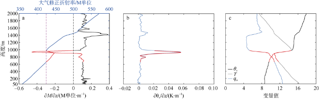
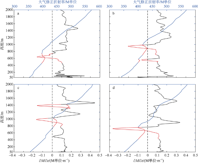
图6 12月15日02时6号探空器观测到的大气修正折射率M (蓝线)及垂直梯度(黑线和红线)的垂直廓线(a)、虚位温垂直梯度廓线($\partial {{\theta }_{\text{v}}}/\partial z$, 单位: K∙m–1)(b)和虚位温 ${{\theta }_{\text{v}}}$减去290K后结果(黑线和红线)、温度T减去8℃后结果(灰线和红线)以及大气比湿qa (浅蓝线和红线, 单位: ×10–3kg∙kg–1)(c)廓线红色为大气悬空波导层(ΔM>1M单位)。图b变量值表示 $\partial {{\theta }_{\text{v}}}/\partial z$的大小; 图c变量值表示经同图处理后变量 ${{\theta }_{\text{v}}}$、T和qa的各自大小。图a中红色虚线表示 Fig. 6 (a) Vertical profile of the atmospheric modified refractive index M (blue line) and its vertical gradient (black line) observed at 02:00 on December 15th; (b) Vertical profile of the virtual potential temperature gradient (units: K∙m-1); (c) Vertical profile of the virtual potential temperature (minus 290K, black line), temperature (minus 8 ℃, gray line), and specific humidity (units: ×10-3kg∙kg-1, blue line). The red and magenta painted parts on the profiles are the stable elevated duct layer identified by ΔM > 1 M-unit |
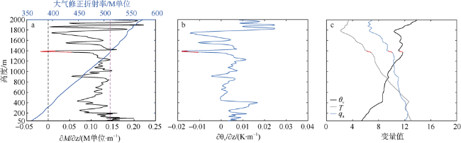
图7 12月22日01时27号探空器观测到的大气修正折射率M (蓝线)及垂直梯度(黑线和红线)的垂直廓线(a)、虚位温垂直梯度廓线($\partial {{\theta }_{\text{v}}}/\partial z$, 单位: K∙m–1)(b)和虚位温 ${{\theta }_{\text{v}}}$减去290K后结果(黑线和红线)、温度T减去8℃后结果(灰线和红线)以及比湿qa (浅蓝线和红线, 单位: ×10–3kg∙kg–1)(c)廓线涂红部分为波导层, 但ΔM>1M单位。图b变量值表示 $\partial {{\theta }_{\text{v}}}/\partial z$的大小; 图c变量值表示变量 ${{\theta }_{\text{v}}}$-290K, T-8℃和qa×10–3的值。图a中红色虚线表示 Fig. 7 (a) Vertical profile of the atmospheric modified refractive index M (blue line) and its vertical gradient (black line) observed at 01:00 on December 22nd; (b) Vertical profile of the virtual potential temperature gradient (units: K∙m-1); (c) Vertical profile of the virtual potential temperature (minus 290K, black line), temperature (minus 8 ℃, gray line), and specific humidity (units: ×10-3kg∙kg-1, blue line). The red painted parts on the profiles are the duct layer but ΔM > 1 M-unit |
图8 12月13日至21日日平均925hPa天气图a. 12月13日; b. 12月15日; c. 12月17日; d. 12月19日; e. 12月21日。蓝线为位势高度(单位: m), 绿色线为温度(单位: K), 灰色线为岸界线。该图基于国家测绘地理信息局标准地图服务网站下载的审图号为GS(2016)1552的标准地图制作 Fig. 8 Daily average weather map of 925 hPa from December 13th to 21st. (a) December 13th; (b) December 15th; (c) December17th; (d) December 19th; (e) December 21st. The coloring is relative humidity, the blue line is the geopotential height, the green line is the temperature, and the gray line is coastline |
图9 |
图10 12月13日至21日日平均地面天气图a. 12月13日; b. 12月15日; c. 12月17日; d. 12月19日; e. 12月21日。填色为相对湿度, 蓝线为温度, 灰线为岸界线。该图基于国家测绘地理信息局标准地图服务网站下载的审图号为GS(2016)1552的标准地图制作 Fig. 10 Daily average weather map of surface from December 13th to 21st. (a) December 13th; (b) December 15th; (c) December 17th; (d) December 19th; (e) December 21st. The coloring is relative humidity, the blue line is the temperature, and the gray line is coastline |
图11 12月15日08时至16日02时在 |
图12 12月21日07时至20时在 |
| [1] |
陈莉, 高山红, 康士峰, 等, 2011. 中国近海蒸发波导的数值模拟与预报研究[J]. 中国海洋大学学报, 41(1-2): 1-8.
|
| [2] |
成印河, 周生启, 王东晓, 等, 2013a. 夏季风爆发对南海南北部低空大气波导的影响[J]. 热带海洋学报, 32(3): 1-8.
|
| [3] |
成印河, 周生启, 王东晓, 2013b. 海上大气波导研究进展[J]. 地球科学进展, 28(3): 318-326.
|
| [4] |
丁菊丽, 费建芳, 黄小刚, 等, 2009. 南海、东海蒸发波导出现规律的对比分析[J]. 电波科学学报, 24(6): 1018-1023.
|
| [5] |
丁轩茹, 管兆勇, 成印河, 等, 2012. 1998年季风试验期间南海蒸发波导特征分析[J]. 热带气象学报, 28(6): 905-910.
|
| [6] |
胡晓华, 费建芳, 张翔, 等, 2007. 气象条件对大气波导的影响[J]. 气象科学, 27(3): 349-354.
|
| [7] |
胡晓华, 费建芳, 张翔, 等, 2008. 一次大气波导过程的数值模拟[J]. 气象科学, 28(3): 294-300.
|
| [8] |
黄小龙, 经志友, 郑瑞玺, 等, 2020. 南海西部夏季上升流锋面的次中尺度特征分析[J]. 热带海洋学报, 39(3): 1-9.
|
| [9] |
康士峰, 张玉生, 王洪光, 2014. 对流层大气波导[M]. 北京: 科学出版社:48-49.
|
| [10] |
蔺发军, 刘成国, 成思, 等, 2005. 海上大气波导的统计分析[J]. 电波科学学报, 20(1): 64-68.
|
| [11] |
蔺发军, 王红光, 林乐科, 等. 2007. 风向对蒸发波导环境特性影响的研究[J]. 电波科学学报, 22(3): 410-413.
|
| [12] |
刘成国, 潘中伟, 郭丽, 1996. 中国低空大气波导出现概率和波导特征量的统计分析[J]. 电波科学学报, 11(2): 60-66.
|
| [13] |
邱春华, 崔永生, 胡诗琪, 等, 2017. 基于融合遥感数据的广东沿岸温度锋面的季节变化研究[J]. 热带海洋学报, 36(5): 16-23.
|
| [14] |
|
| [15] |
|
| [16] |
|
| [17] |
|
| [18] |
|
| [19] |
|
| [20] |
|
| [21] |
|
| [22] |
|
/
| 〈 |
|
〉 |


