
Journal of Tropical Oceanography >
An ocean current direction correction method for high-frequency surface wave radars based on CNN-LSTM
Copy editor: LIN Qiang
Received date: 2024-09-12
Revised date: 2024-10-29
Online published: 2024-11-04
Supported by
Southern Marine Science and Engineering Guangdong Laboratory (Zhuhai)(SML2020SP009)
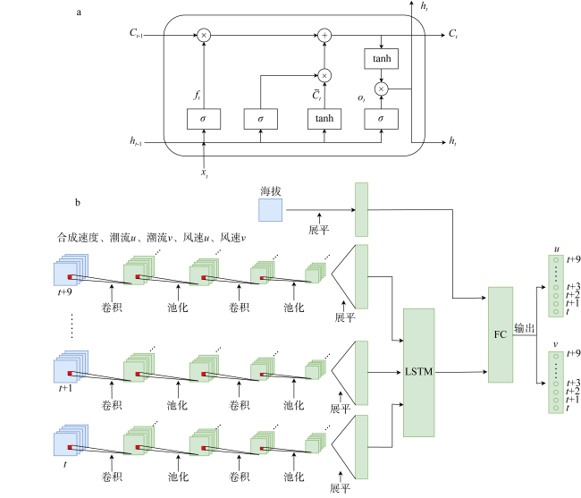
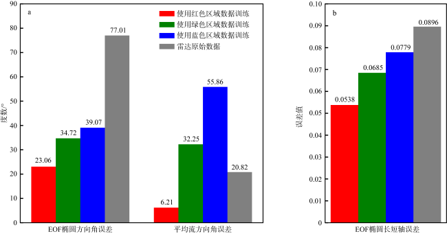
High-frequency surface wave radars often encounter interference from coastal topography and islands when detecting nearshore areas, leading to significant errors in the synthesized ocean current directions from radar data. Traditional high-frequency surface wave radar inversion algorithms do not account for the impact of these physical factors. To address this issue, leveraging the strengths of convolutional neural networks (CNN) and long short-term memory (LSTM) neural networks, this paper introduces a hybrid CNN-LSTM model. This model incorporates data on sea surface wind, tide, and elevation, allowing for the refinement of ocean current directions obtained from radar measurements. The experimental results show that the CNN-LSTM model, when combined with physical oceanographic factors, can effectively improve the quality of radar-detected ocean current data in areas affected by topography, significantly enhancing the accuracy of the synthesized ocean current direction. After model correction, compared to the original radar data, the directional angle error of the empirical orthogonal function ellipse decreased from 77.10° to 23.06°, the error of the ellipse’s major and minor axes decreased from 0.0896 to 0.0538, and the average flow directional angle error of the ocean currents decreased from 20.82° to 6.21°.
XU Yi , WEI Jun , WEI Chunlei , YANG Fan . An ocean current direction correction method for high-frequency surface wave radars based on CNN-LSTM[J]. Journal of Tropical Oceanography, 2025 , 44(3) : 24 -35 . DOI: 10.11978/2024176
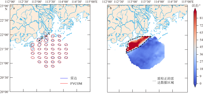
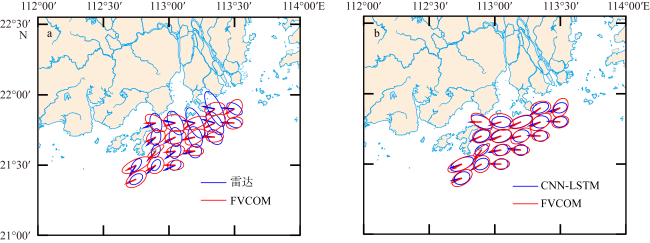
图3 雷达与模式数据EOF椭圆对比图(a)及两者的方向角误差(b)蓝色为雷达数据, 红色为模式数据, 数据点以经度0.25°、纬度0.15°的间隔绘制; 用“★”标记点A(21°57′N, 113°21′E)和点B(21°48′N, 113°06′E) Fig. 3 EOF ellipses comparison between radar and model data (a) and their directional angle errors (b). Blue represents radar data, red represents model data, and the data points are plotted at intervals of 0.25° longitude and 0.15° latitude. Points A (21°57′N, 113°21′E) and B (21°48′N, 113°06′E) are marked with “★” |
图5 原始雷达数据与模式数据的EOF椭圆对比图(a)及校正后雷达数据与模式数据的EOF椭圆对比图(b)数据点以经度0.15°、纬度0.10°的间隔绘制。a、b中蓝色分别是原始雷达数据和网络模型校正后数据的EOF椭圆, 红色是模式数据的EOF椭圆, 箭头表示平均流方向 Fig. 5 EOF ellipses contrast graph (a) between original radar data and model data and EOF ellipses contrast graph (b) between corrected radar data and model data. Data points are plotted at intervals of 0.15° longitude and 0.10° latitude. In (a) and (b), blue represents the EOF ellipses of the original radar data and the neural network corrected data, respectively, and red represents the EOF ellipses of the model data. The arrows indicate the direction of the mean flow |
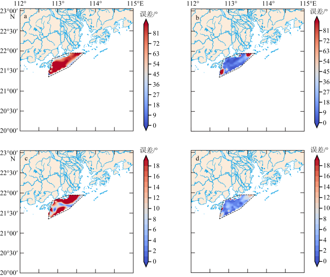
图6 雷达数据校正前(a)和校正后(b)的EOF椭圆方向角误差对比, 以及雷达数据校正前(c)和校正后(d)的平均流方向角误差对比Fig. 6 (a) and (b) are comparison charts of the directional angle errors of EOF ellipses before and after correction of radar data, respectively, and (c) and (d) are comparison charts of the mean flow directional angle errors before and after correction of radar data, respectively |
表1 不同卷积层、隐藏层数量的神经网络模型校正效果对比Tab. 1 Comparison of correction effects of neural network models with different numbers of convolutional layers and hidden layers |
| 卷积层数量 | 隐藏层数量 | 椭圆长短轴误差 | 椭圆方向角误差 | 平均流方向角误差 | 三个指标平均提升幅度 |
|---|---|---|---|---|---|
| 1 | 80 | 0.0767 | 25.31° | 8.66° | 46.65% |
| 1 | 160 | 0.0775 | 25.65° | 8.79° | 45.99% |
| 1 | 240 | 0.0766 | 25.20° | 8.81° | 46.49% |
| 2 | 80 | 0.0558 | 24.67° | 6.14° | 58.73% |
| 2 | 160 | 0.0538 | 23.06° | 6.21° | 60.06% |
| 2 | 240 | 0.0555 | 24.13° | 6.83° | 57.97% |
| 4 | 80 | 0.0535 | 23.61° | 8.52° | 56.24% |
| 4 | 160 | 0.0500 | 23.79° | 8.41° | 57.64% |
| 4 | 240 | 0.0553 | 23.33° | 8.38° | 55.91% |
表2 不同卷积核大小、dropout层失活率的神经网络模型校正效果对比Tab. 2 Comparison of correction effects of neural network models with different convolutional kernel sizes and dropout rates |
| 卷积核大小 | 失活率 | 椭圆长短轴误差 | 椭圆方向角误差 | 平均流方向角误差 | 三个指标平均提升幅度 |
|---|---|---|---|---|---|
| 2 | 0 | 0.0624 | 24.06° | 7.47° | 54.41% |
| 3 | 0 | 0.0538 | 23.06° | 6.21° | 60.06% |
| 4 | 0 | 0.0505 | 23.79° | 7.29° | 59.24% |
| 3 | 0.25 | 0.0593 | 23.17° | 9.31° | 53.00% |
| 3 | 0.5 | 0.0708 | 24.57° | 9.87° | 47.22% |
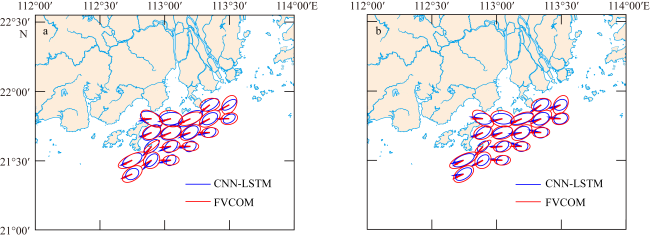
图8 雷达数据经过神经网络模型校正后与模式数据的EOF椭圆对比a. 神经网络模型的输入为雷达海流数据+潮流数据+海拔数据; b. 神经网络模型的输入为雷达海流数据+风速数据+海拔数据, 数据点以经度0.15°、纬度0.10°的间隔绘制 Fig. 8 Comparison of EOF ellipses between neural network corrected radar data and model data. In (a), the input to the neural network model is radar ocean current data + tidal current data + elevation data. In (b), the input to the neural network model is radar ocean current data + wind speed data + elevation data. Data points are plotted at intervals of 0.15° longitude and 0.10° latitude |
表3 神经网络模型敏感性实验的校正效果对比Tab. 3 Comparison of correction effects in sensitivity experiments of the neural network model |
| 实验 | 椭圆长短轴误差 | 椭圆方向角误差 | 平均流方向角误差 |
|---|---|---|---|
| 实验1 | 0.0540 | 35.57° | 8.97° |
| 实验2 | 0.0589 | 26.32° | 10.29° |
| 实验3 | 0.0629 | 28.18° | 10.38° |
| 实验4 | 0.0538 | 23.06° | 6.21° |
| 原始数据 | 0.0896 | 77.01° | 20.82° |
| [1] |
蔡佳佳, 曾玉明, 周浩, 等, 2019. 基于人工神经网络的高频雷达风速反演[J]. 海洋学报, 41(11): 150-155.
|
| [2] |
东松林, 岳显昌, 吴雄斌, 等, 2022. 基于深度学习的高频雷达射频干扰自动识别与抑制[J]. 雷达科学与技术, 20(3): 260-271.
|
| [3] |
吴雄斌, 张兰, 柳剑飞, 2015. 海洋雷达探测技术综述[J]. 海洋技术学报, 34(3): 8-15.
|
| [4] |
于彩彩, 楚晓亮, 王曙曜, 2024. 基于卷积神经网络的高频地波雷达有效波高反演[J]. 海洋科学进展, 42(1): 126-136.
|
| [5] |
周东旭, 孙维康, 付海德, 等, 2023. 三种最新全球海潮模型在中国沿海的精度评估[J]. 海洋科学进展, 41(1): 54-63.
|
| [6] |
|
| [7] |
|
| [8] |
|
| [9] |
|
| [10] |
|
| [11] |
|
| [12] |
|
| [13] |
|
| [14] |
|
| [15] |
|
| [16] |
|
| [17] |
|
| [18] |
|
| [19] |
|
| [20] |
|
| [21] |
|
| [22] |
|
| [23] |
|
| [24] |
|
/
| 〈 |
|
〉 |
