
Journal of Tropical Oceanography >
Retrieving phytoplankton size class from hyperspectral particulate absorption data measured by the ship-based underway flow-through system
Received date: 2018-05-03
Request revised date: 2018-06-14
Online published: 2018-10-13
Supported by
National Natural Science Foundation of China (41776045, 41576030, 41776044)
Fundamental Research Funds for the Central Universities (2017B06714)
Open Project Program of the State Key Laboratory of Tropical Oceanography (LTOZZ1602)
Science and Technology Program of Guangzhou, China (201607020041)
Copyright
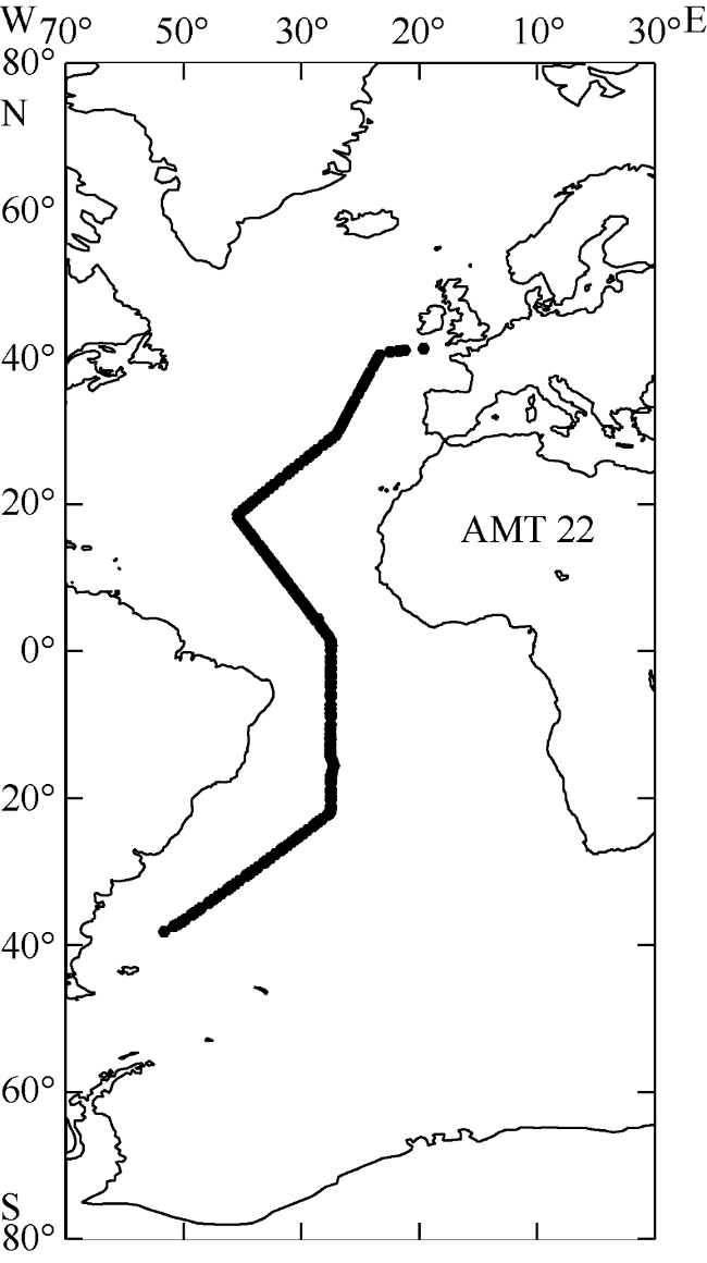
Retrieving of phytoplankton groups from hyperspectral optical data has been a hot topic in recent years for studies of marine optics and ocean color remote sensing. In this paper, based on the hyperspectral particulate absorption data (ap(λ)) measured by the ship’s flow-through system during the Atlantic Meridional Transect (AMT) cruise, two models were proposed and compared for estimating phytoplankton size class (PSC) from the ap(λ) spectra. An algorithm that defines phytoplankton pigment absorption as a sum of Gaussian functions was used for decomposing the total particulate absorption, and a partial least squares model (PLS_model) was developed for estimating PSC using the Gaussian magnitudes at specific wavelengths. Another model (3component_model) is a modified abundance-based model proposed by
WANG Guifen , XU Wenlong , ZHOU Wen , XU Zhantang , CAO Wenxi . Retrieving phytoplankton size class from hyperspectral particulate absorption data measured by the ship-based underway flow-through system[J]. Journal of Tropical Oceanography, 2018 , 37(5) : 50 -61 . DOI: 10.11978/2018049
Fig. 1 Cruise track of AMT22 for underway hyperspectral measurements图1 大西洋经向断面航次(AMT 22)调查站位分布图 |
Tab. 1 Statistical test parameters and calculation formulas表1 统计参数的简介及计算公式 |
| 符号 | 描述 | 计算公式 |
|---|---|---|
| r | 皮尔逊相关系数 | $\frac{1}{N-1}\sum\limits_{i=1}^{N}{\left[ \frac{C_{i}^{\mathrm{M}}-\left( \frac{1}{N}\sum\nolimits_{j\mathrm{=1}}^{N}{C_{j}^{\mathrm{M}}} \right)}{{{\left\{ \frac{\mathrm{1}}{N-\mathrm{1}}\sum\nolimits_{k\mathrm{=1}}^{N}{\left[ C_{k}^{\mathrm{M}}-\left( \frac{\mathrm{1}}{N}\sum\nolimits_{i}^{N}{C_{i}^{\mathrm{M}}} \right) \right]} \right\}}^{1/2}}} \right]}\left[ \frac{C_{i}^{\mathrm{E}}-\left( \frac{1}{N}\sum\nolimits_{m\mathrm{=1}}^{N}{C_{m}^{\mathrm{E}}} \right)}{{{\left\{ \frac{\mathrm{1}}{N-\mathrm{1}}\sum\nolimits_{n\mathrm{=1}}^{N}{\left[ C_{n}^{\mathrm{E}}-\left( \frac{\mathrm{1}}{N}\sum\nolimits_{0}^{N}{C_{0}^{\mathrm{E}}} \right) \right]} \right\}}^{1/2}}} \right]$ |
| ψ/(mg·m-3) | 均方根差 | ${{\left[ \frac{\mathrm{1}}{N}\sum\limits_{i\mathrm{=1}}^{N}{{{\left( C_{i}^{\mathrm{E}}-C_{i}^{\mathrm{M}} \right)}^{\mathrm{2}}}} \right]}^{1/2}}$ |
| δ/(mg·m-3) | 偏差 | $\frac{\mathrm{1}}{N}\sum\limits_{i\mathrm{=1}}^{N}{\left( C_{i}^{\mathrm{E}}-C_{i}^{\mathrm{M}} \right)}$ |
| R2 | 决定系数 | $\mathrm{1}-\frac{\sum\nolimits_{i\mathrm{=1}}^{N}{{{\left( C_{i}^{\mathrm{E}}-C_{i}^{\mathrm{M}} \right)}^{\mathrm{2}}}}}{\sum\nolimits_{i\mathrm{=1}}^{N}{{{\left( C_{i}^{\mathrm{M}}-\left( \frac{\mathrm{1}}{N}\sum\nolimits_{i\mathrm{=1}}^{N}{C_{i}^{\mathrm{M}}} \right) \right)}^{\mathrm{2}}}}}$ |
| ME/% | 平均相对偏差 | $\frac{\mathrm{1}}{N}\sum\limits_{i\mathrm{=1}}^{N}{\left( \frac{\left| C_{i}^{\mathrm{E}}-C_{i}^{\mathrm{M}} \right|}{C_{i}^{\mathrm{M}}} \right)\times \mathrm{100}}$ |
注: C为叶绿素浓度, 上标M和E分别表示实测数据和模型估测值, N为样本个数, i、j、k表征不同样本, r、R2为无量纲量 |
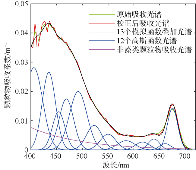
Fig. 2 Example of Gaussian decomposition for particulate absorption measured with AC-S图2 AC-S测量颗粒物吸收系数的高斯分解示例 |
Tab. 2 Center wavelengths (peak location) and widths (σ) of Gaussian functions used as input for spectral decomposition followed Chase et al (2013)表2 颗粒物吸收光谱分解时选取的高斯函数的中心波长及带宽(Chase et al, 2013) |
| 高斯分解参数 | ||||||||||||
|---|---|---|---|---|---|---|---|---|---|---|---|---|
| 中心波长/nm | 406 | 435 | 454 | 469 | 492 | 523 | 550 | 585 | 617 | 639 | 661 | 675 |
| 带宽σ/nm | 17 | 13 | 12 | 14 | 17 | 15 | 15 | 17 | 14 | 11 | 11 | 10 |
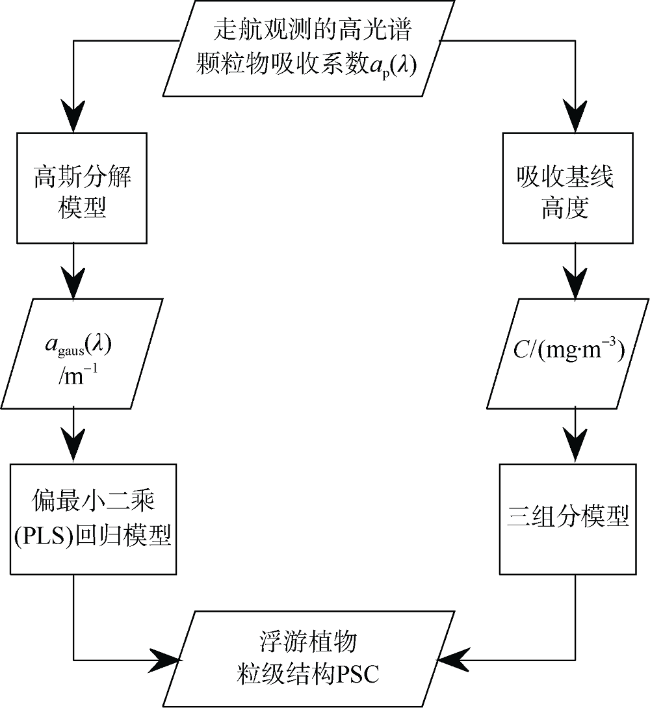
Fig. 3 Schematic of the data and processing steps to estimate phytoplankton size class图3 反演浮游植物粒级结构模型的流程图 |
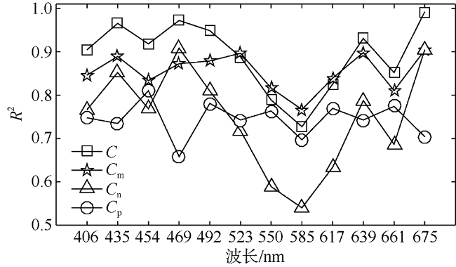
Fig. 4 Determination coefficients (R2) for linear correlations between chlorophyll a concentration (C, Cm, Cn, Cp, mg·m-3) and decomposed Gaussian bands at difference peak locations图 4 不同波段高斯峰强度与总叶绿素a浓度(C)及分粒级叶绿素a浓度(Cm, Cn, Cp, 单位: mg·m-3)之间线性相关的决定系数R2分布 |
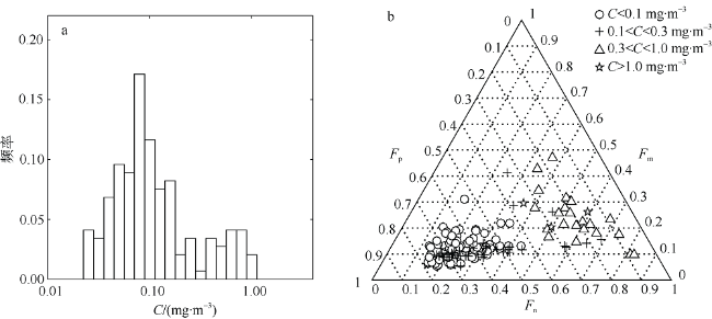
Fig. 5 Variations of phytoplankton size classes. (a) Frequency distribution of total chlorophyll a concentration in AMT22 (N=145), and (b) ternary plot of the fractions of three phytoplankton size classes (Fm, Fn, Fp), with the marker showing different C ranges图5 浮游植物粒级结构的分布图 |
Tab. 3 Parameters for PLS regression model trained with HPLC pigment measurements and Gaussian bands (N=73)表3 HPLC分析的色素浓度与高斯带之间关系建立的偏最小二乘(PLS)回归模型中的参数(N=73) |
| 主成分 个数 | 相关系数 | 均方根差 | 线性拟合 斜率 | 线性拟 合截距 | |
|---|---|---|---|---|---|
| Cp | 3 | 0.743 | 0.025 | 0.596 | -0.511 |
| Cn | 4 | 0.935 | 0.025 | 0.888 | -0.163 |
| Cm | 2 | 0.916 | 0.018 | 0.854 | -0.282 |
| C | 3 | 0.973 | 0.022 | 0.946 | -0.051 |
Tab. 4 Parameter values obtained from the three- component model, compared with Brewin et al (2010)表4 基于总叶绿素a浓度建立的三组分模型参数(与Brewin 等(2010)模型比较) |
| $C_{\mathrm{p,n}}^{\mathrm{m}}$ | Sp, n | $C_{\mathrm{p}}^{\mathrm{m}}$ | Sp | RMSEp,n | RMSEp | |
|---|---|---|---|---|---|---|
| 本文 | 2.1882 | 0.4050 | 0.1557 | 4.7234 | 0.021 | 0.041 |
| Brewin 等(2010) | 1.057 | 0.851 | 0.107 | 6.801 | 0.045 | 0.048 |
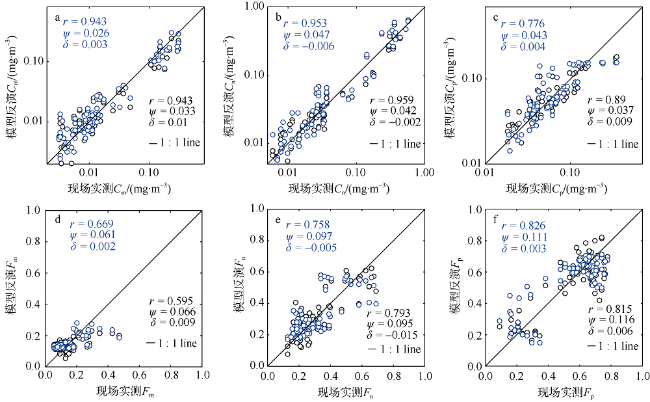
Fig. 6 Comparison between predicated and measured concentrations and fractions with three phytoplankton size classes from the validation data set (N=72). Black circle represents the PLS regression model result, and blue circle represents the three-component model result. The 1:1 ratio is shown as a solid line图6 采用验证数据集(N=72)反演得到的各粒级浮游植物浓度及比例与实测数据的比较(黑色代表PLS回归模型, 蓝色代表三组分模型), 黑色实线为1:1线 |
Tab. 5 Comparison of statistical parameters between HPLC-measured and model-predicted values based on validation data set (N=72)表5 基于独立数据集(N=72)验证三个粒级浮游植物色素浓度及比例的统计参数分布 |
| 参量 | r | Ψ | δ | ME/% | |
|---|---|---|---|---|---|
| 偏最小二乘 回归模型 | Cp | 0.890 | 0.037 | 0.009 | 28.4 |
| Cn | 0.959 | 0.042 | -0.002 | 31.9 | |
| Cm | 0.943 | 0.033 | 0.010 | 41.0 | |
| Fp | 0.815 | 0.116 | 0.006 | 23.4 | |
| Fn | 0.793 | 0.095 | -0.015 | 26.8 | |
| Fm | 0.595 | 0.066 | 0.009 | 38.4 | |
| 三组分 模型 | Cp | 0.776 | 0.043 | 0.004 | 31.0 |
| Cn | 0.953 | 0.047 | -0.006 | 35.9 | |
| Cm | 0.943 | 0.026 | 0.003 | 37.7 | |
| Fp | 0.826 | 0.111 | 0.003 | 24.9 | |
| Fn | 0.758 | 0.097 | -0.005 | 25.3 | |
| Fm | 0.669 | 0.061 | 0.002 | 33.1 |
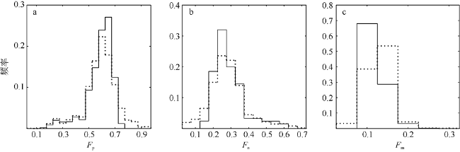
Fig. 7 Frequency distributions of Fp, Fn and Fm determined from the underway flow-through system data set. Black line represents the PLS regression model result, and dotted line represents the three-component model图7 采用走航观测数据比较PLS回归模型(黑线)与三组分模型(点线)反演得到的浮游植物粒级结构频率分布 |
The authors have declared that no competing interests exist.
| [1] |
|
| [2] |
|
| [3] |
|
| [4] |
|
| [5] |
|
| [6] |
|
| [7] |
|
| [8] |
|
| [9] |
|
| [10] |
|
| [11] |
|
| [12] |
|
| [13] |
|
| [14] |
|
| [15] |
|
| [16] |
|
| [17] |
|
| [18] |
|
| [19] |
|
| [20] |
|
| [21] |
IOCCG, 2014. Phytoplankton functional types from space[R]//SATHYENDRANATH S. Reports of the International Ocean-Colour Coordinating Group, No. 15. Dartmouth, Canada: IOCCG.
|
| [22] |
|
| [23] |
|
| [24] |
|
| [25] |
|
| [26] |
|
| [27] |
|
| [28] |
|
| [29] |
|
| [30] |
|
| [31] |
|
| [32] |
|
| [33] |
|
| [34] |
|
| [35] |
|
/
| 〈 |
|
〉 |
