
Journal of Tropical Oceanography ›› 2022, Vol. 41 ›› Issue (2): 1-15.doi: 10.11978/2021070CSTR: 32234.14.2021070
• Marine Hydrology • Next Articles
Research and application of global three-dimensional thermohaline reconstruction technology based on neural network
NIE Wangchen1( ), WANG Xidong1,2(), CHEN Zhiqiang1, HE Zikang1, FAN Kaigui1
- 1. Key Laboratory of Research on Marine Hazards Forecasting, Ministry of Natural Resources, College of Oceanography, Hohai University, Nanjing 210098, China
2. Southern Marine Science and Engineering Guangdong Laboratory (Zhuhai), Zhuhai 519000, China
-
Received:2021-06-06Revised:2021-07-28Online:2022-03-10Published:2021-08-16 -
Contact:WANG Xidong E-mail:191311040024@hhu.edu.cn;191311040024@hhu.edu.cn;xidong_wang@hhu.edu.cn -
Supported by:National Natural Science Foundation of China(41776004)
CLC Number:
- P731.1
Cite this article
NIE Wangchen, WANG Xidong, CHEN Zhiqiang, HE Zikang, FAN Kaigui. Research and application of global three-dimensional thermohaline reconstruction technology based on neural network[J].Journal of Tropical Oceanography, 2022, 41(2): 1-15.
share this article
Add to citation manager EndNote|Reference Manager|ProCite|BibTeX|RefWorks
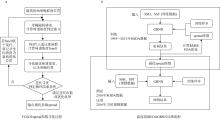
Fig. 1
The process of FOA and the process of FOAGRNN reconstruction of temperature and salinity field. The flow chart on the left corresponds to the FOA optimization mini-cycle on the right, S value corresponds to spread parameter, Smell corresponds to RMSE of reconstruction results and training samples; When condition is met, the end of the cycle, and outputs the optimal parameters of spread"

Fig. 1
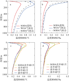
Fig. 2
The changes of RMSE error between original field and SODA reconstruction results/climate state data with water depth. (a) Temperature field, in the worldwide scale and 2016 average; (b) salinity field, in the worldwide scale and 2016 average; (c) RMSE of temperature field between SODA original field and reconstructed results in the Northern/Southern Hemisphere and January/July; (d) RMSE of salinity field between SODA original field and reconstructed results in the Northern/Southern Hemisphere and January/July"
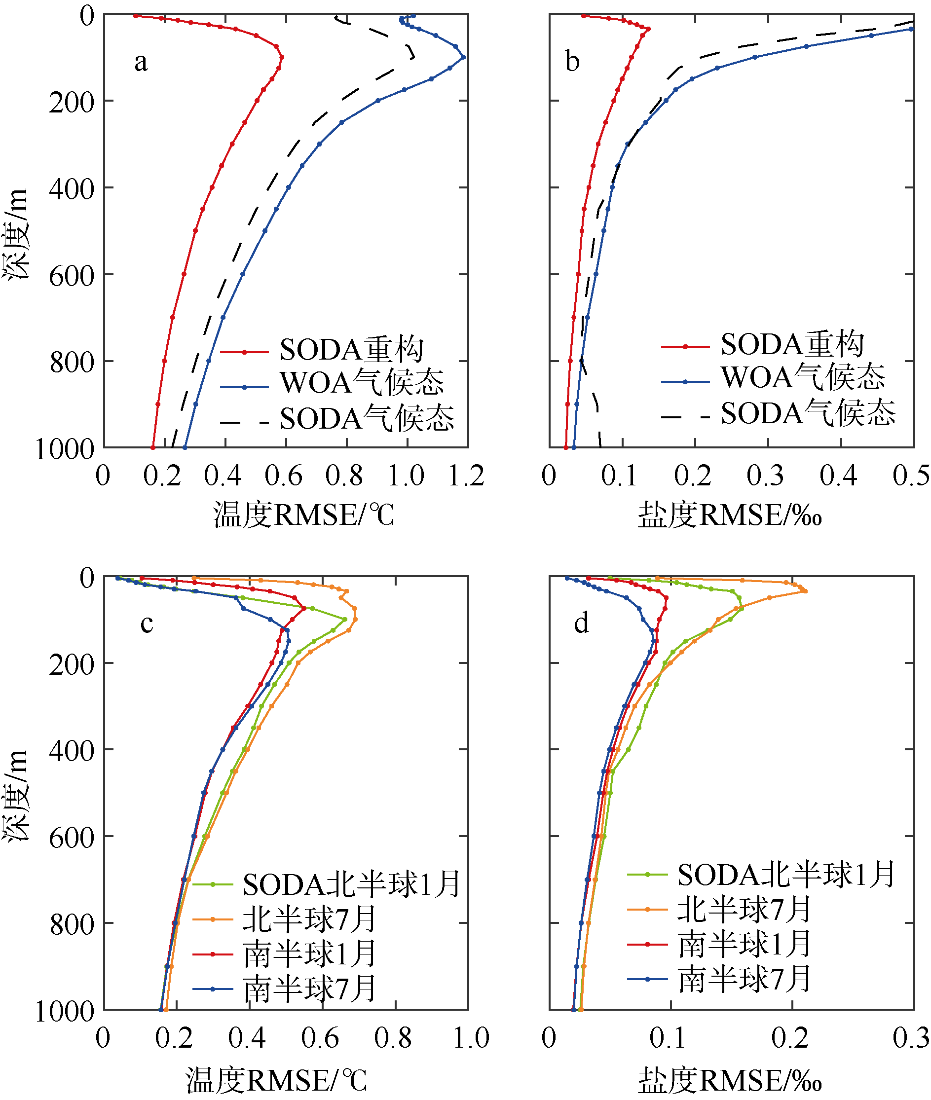
Fig. 2
Fig. 3
The selected representative area and Argo floats tracks. NP (North Pacific): 150°—170°E, 30°—40°N; NA (North Atlantic): 40°—20°W, 40°—50°N; EQWP (Equatorial Western Pacific): 170°—170°W, 10°S—0; EQEP (Equatorial Eastern Pacific): 110°—90°W, 10°S—0; SI (Southern indian Ocean): 50°—70°E, 40°—30°S; ANT (Antarctic Ocean): 120°—60°W, 65°—55°S. Argo float ID numbers: (1) 5902460, (2) 5903130, (3) 5905167, (4) 5904090, (5) 2902653, and (6) 6901584. These red curves are the Argo buoy track, and these black dots are the starting point of the tracks; the number of float profiles is between 72 and 146"

Fig. 3
Tab. 1
Vertical MRMSE between original and reconstructed SODA field/ climate state in each region"
| 重构温度 MRMSE/℃ | WOA气候态MRMSE/℃ | SODA气候态MRMSE/℃ | 重构盐度MRMSE/‰ | WOA气候态MRMSE/‰ | SODA气候态MRMSE/‰ | |
|---|---|---|---|---|---|---|
| 北太平洋 | 0.37 | 1.07 | 0.97 | 0.05 | 0.11 | 0.11 |
| 北大西洋 | 0.41 | 0.88 | 0.86 | 0.07 | 0.17 | 0.16 |
| 赤道西太 | 0.30 | 0.89 | 0.72 | 0.07 | 0.24 | 0.20 |
| 赤道东太 | 0.37 | 0.85 | 0.79 | 0.04 | 0.09 | 0.08 |
| 南印度洋 | 0.29 | 0.61 | 0.56 | 0.04 | 0.09 | 0.11 |
| 南大洋 | 0.23 | 0.65 | 0.61 | 0.04 | 0.12 | 0.12 |
| 平均 | 0.33±0.06 | 0.83±0.13 | 0.75±0.12 | 0.05±0.01 | 0.14±0.05 | 0.13±0.03 |
Tab. 1
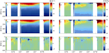
Fig. 4
Distribution of temperature and salinity field in a zonal section. (a) and (d). SODA reconstructed temperature/salt profiles; (b) and (e). SODA raw data temperature/salt profiles; (c) and (f). their difference. The cross profile is along a latitude passing 00°15′E, and the time is January 29, 2016. The blank space represents land"
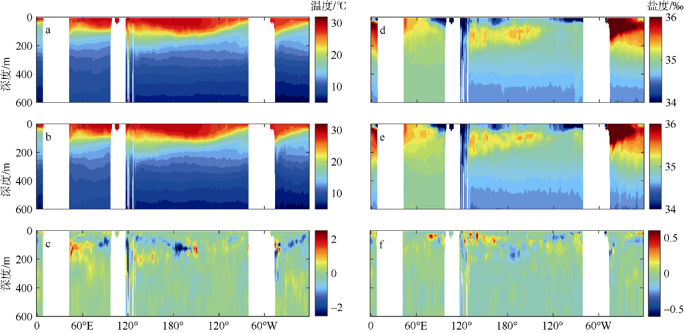
Fig. 4
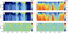
Fig. 5
Distribution of temperature and salinity field in a zonal section. (a) and (d). SODA reconstructed temperature/salt profiles; (b) and (e). SODA raw data temperature/salt profiles; (c) and (f). their difference. The cross profile is along a latitude passing 60°S, and the time is January 29, 2016"

Fig. 5
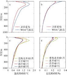
Fig. 6
Changes of RMSE between Argo field observation data, satellite data reconstruction results/WOA climate state data with water depth. (a) Temperature field, in the worldwide scale and 2016 average; (b) salinity field, in the worldwide scale and 2016 average; (c) temperature field reconstruction error, in the Northern/Southern Hemisphere and January/July; (d) salinity field reconstruction error, in the Northern/Southern Hemisphere and January/July"

Fig. 6
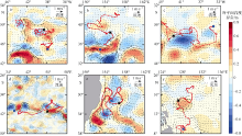
Fig. 7
Argo float track and background field. Argo float number. (a) 5902460; (b) 5904090; (c) 5903130; (d) 6901584; (e) 5905167; (f) 2902653. The red curve is float track, and the blue cross is the starting point of the track, and black cross is the corresponding moment of the surface flow field and SLA"
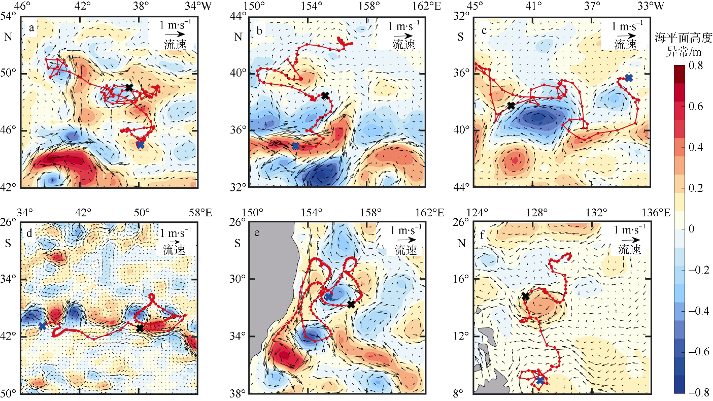
Fig. 7

Fig. 8
Argo float 5902460, located in the North Atlantic Ocean. (a) Argo observed temperature field; (b) satellite data reconstruction temperature field; (c) Argo observed salinity field; (d) satellite data reconstruction salinity field; (e) The Argo/satellite reconstruction/WOA13 temperature profile at the time corresponding to the dotted line in fig. a; (f) salinity field; (g) RMSE of observed temperature field and reconstructed temperature field/WOA13 climate state; (h) salinity field; (i) steric height calculated by Argo profile and reconstructed profile. The red vertical line in fig. a is the corresponding time of the black cross in fig. 7"
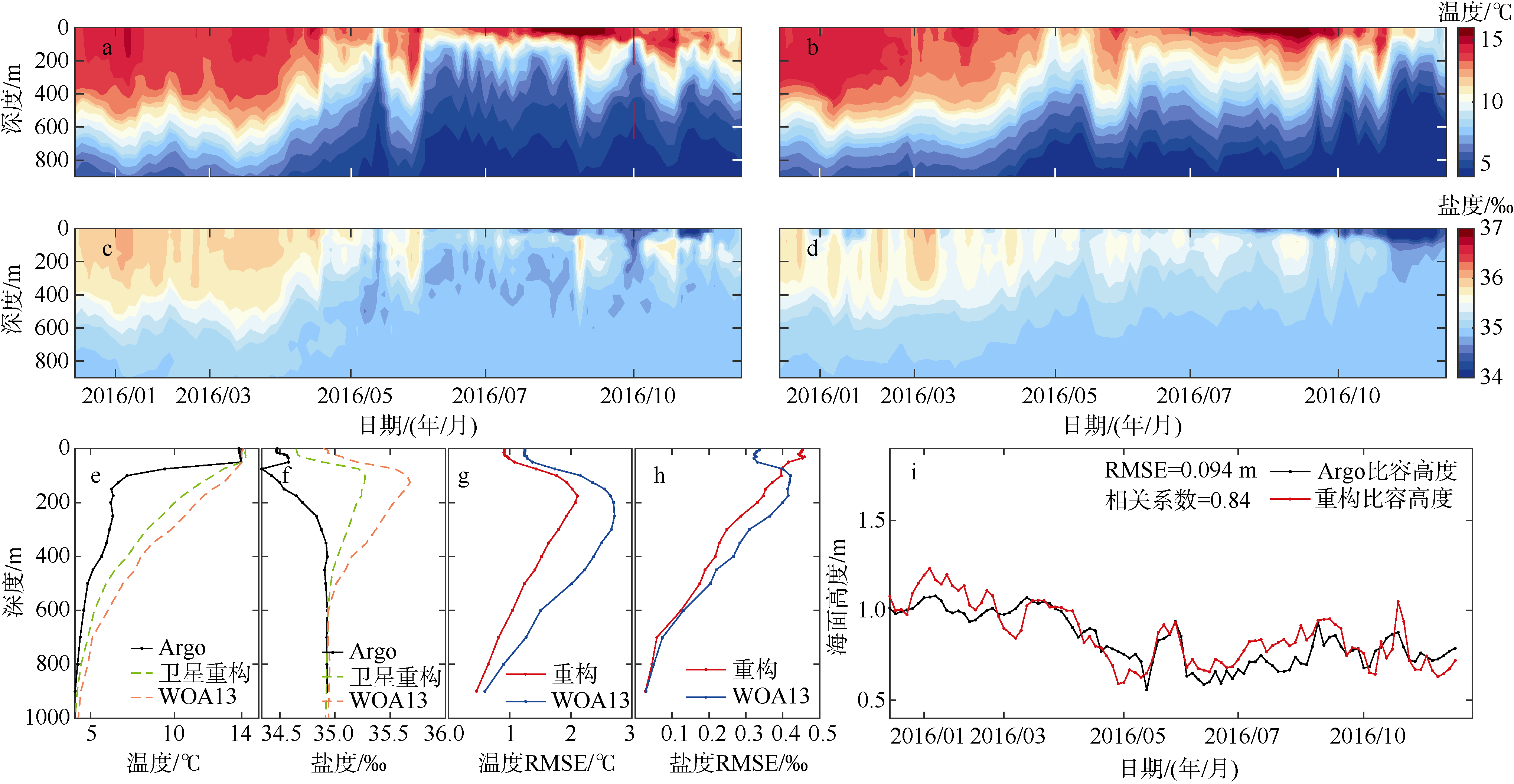
Fig. 8

Fig. 9
Argo float 5904090, located in the Kuroshio extension. (a) Argo observed temperature field; (b) satellite data reconstruction temperature field; (c) Argo observed salinity field; (d) satellite data reconstruction salinity field; (e) The Argo/satellite reconstruction/WOA13 temperature profile at the time corresponding to the dotted line in fig. a; (f) salinity field; (g) RMSE of observed temperature field and reconstructed temperature field/WOA13 climate state; (h) salinity field; (i) steric height calculated by Argo profile and reconstructed profile. The red vertical line in fig. a is the corresponding time of the black cross in fig. 7"
Fig. 9
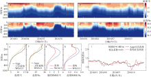
Fig. 10
Argo float 5903130, located in the South Atlantic Ocean. (a) Argo observed temperature field; (b) satellite data reconstruction temperature field; (c) Argo observed salinity field; (d) satellite data reconstruction salinity field; (e) The Argo/satellite reconstruction/WOA13 temperature profile at the time corresponding to the dotted line in fig. a; (f) salinity field; (g) RMSE of observed temperature field and reconstructed temperature field/WOA13 climate state; (h) salinity field; (i) steric height calculated by Argo profile and reconstructed profile. The red vertical line in fig. a is the corresponding time of the black cross in fig. 7"

Fig. 10
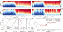
Fig. 11
Argo float 6901584, located in the southern Indian Ocean. (a) Argo observed temperature field; (b) satellite data reconstruction temperature field; (c) Argo observed salinity field; (d) satellite data reconstruction salinity field; (e) The Argo/satellite reconstruction/WOA13 temperature profile at the time corresponding to the dotted line in fig. a; (f) salinity field; (g) RMSE of observed temperature field and reconstructed temperature field/WOA13 climate state; (h) salinity field; (i) steric height calculated by Argo profile and reconstructed profile. The red vertical line in fig. a is the corresponding time of the black cross in fig. 7"

Fig. 11
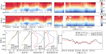
Fig. 12
Argo float 5905167, located in the East Australian Current. (a) Argo observed temperature field; (b) satellite data reconstruction temperature field; (c) Argo observed salinity field; (d) satellite data reconstruction salinity field; (e) The Argo/satellite reconstruction/WOA13 temperature profile at the time corresponding to the dotted line in fig. a; (f) salinity field; (g) RMSE of observed temperature field and reconstructed temperature field/WOA13 climate state; (h) salinity field; (i) steric height calculated by Argo profile and reconstructed profile. The blank in (a) and (c) is caused by the lack of Argo data; The blank in (b), (d) and the curve discontinuity in (i) are caused by the lack of satellite data. The red vertical line in fig. a is the corresponding time of the black cross in fig. 7"
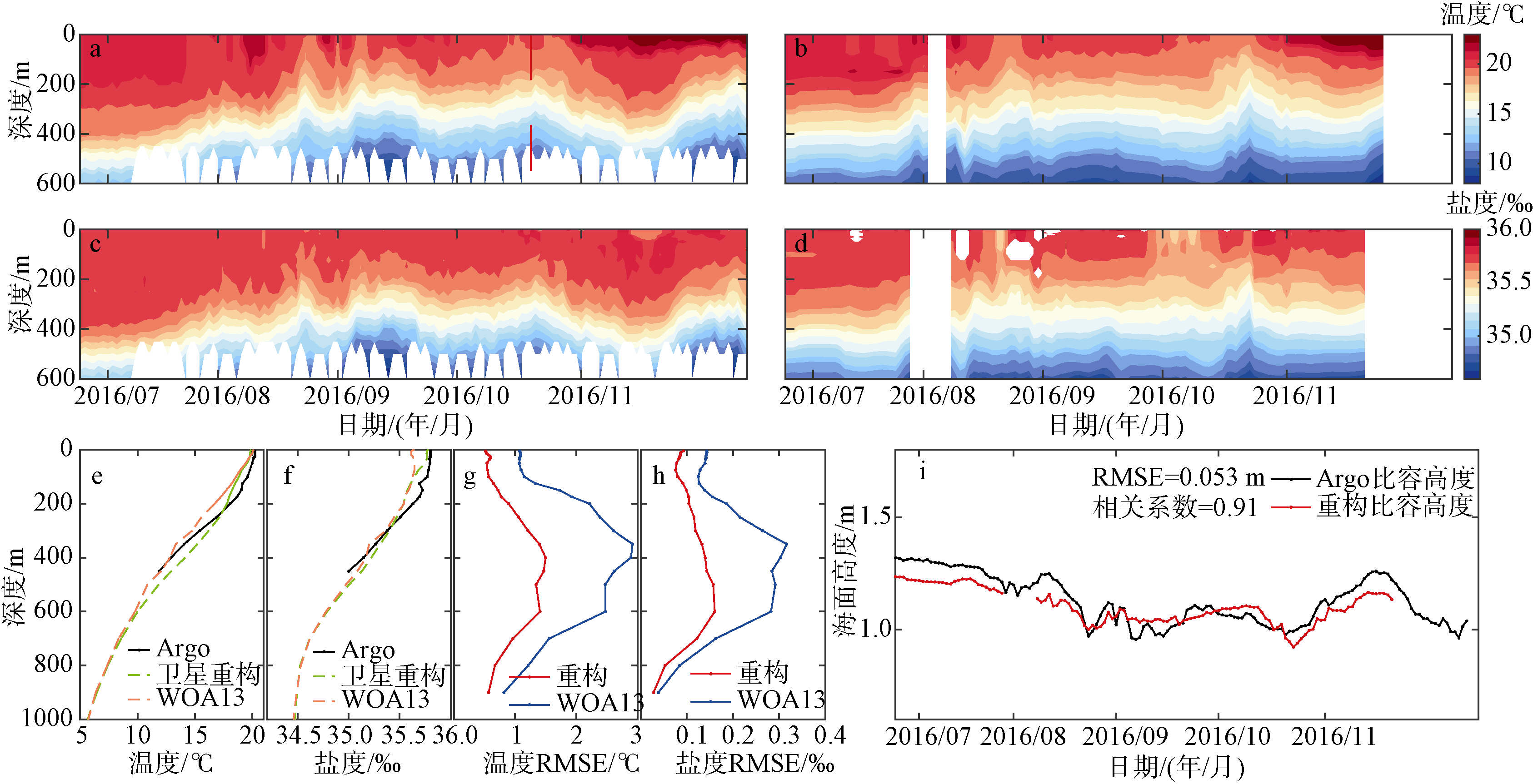
Fig. 12
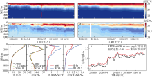
Fig. 13
Argo float 2902653, located near the western Pacific. (a) Argo observed temperature field; (b) satellite data reconstruction temperature field; (c) Argo observed salinity field; (d) satellite data reconstruction salinity field; (e) The Argo/satellite reconstruction/WOA13 temperature profile at the time corresponding to the dotted line in fig. a; (f) salinity field; (g) RMSE of observed temperature field and reconstructed temperature field/WOA13 climate state; (h) salinity field; (i) steric height calculated by Argo profile and reconstructed profile. The blank in (d) and the curve discontinuity in (i) are caused by the lack of satellite data. The red vertical line in fig. a is the corresponding time of the black cross in fig. 7"
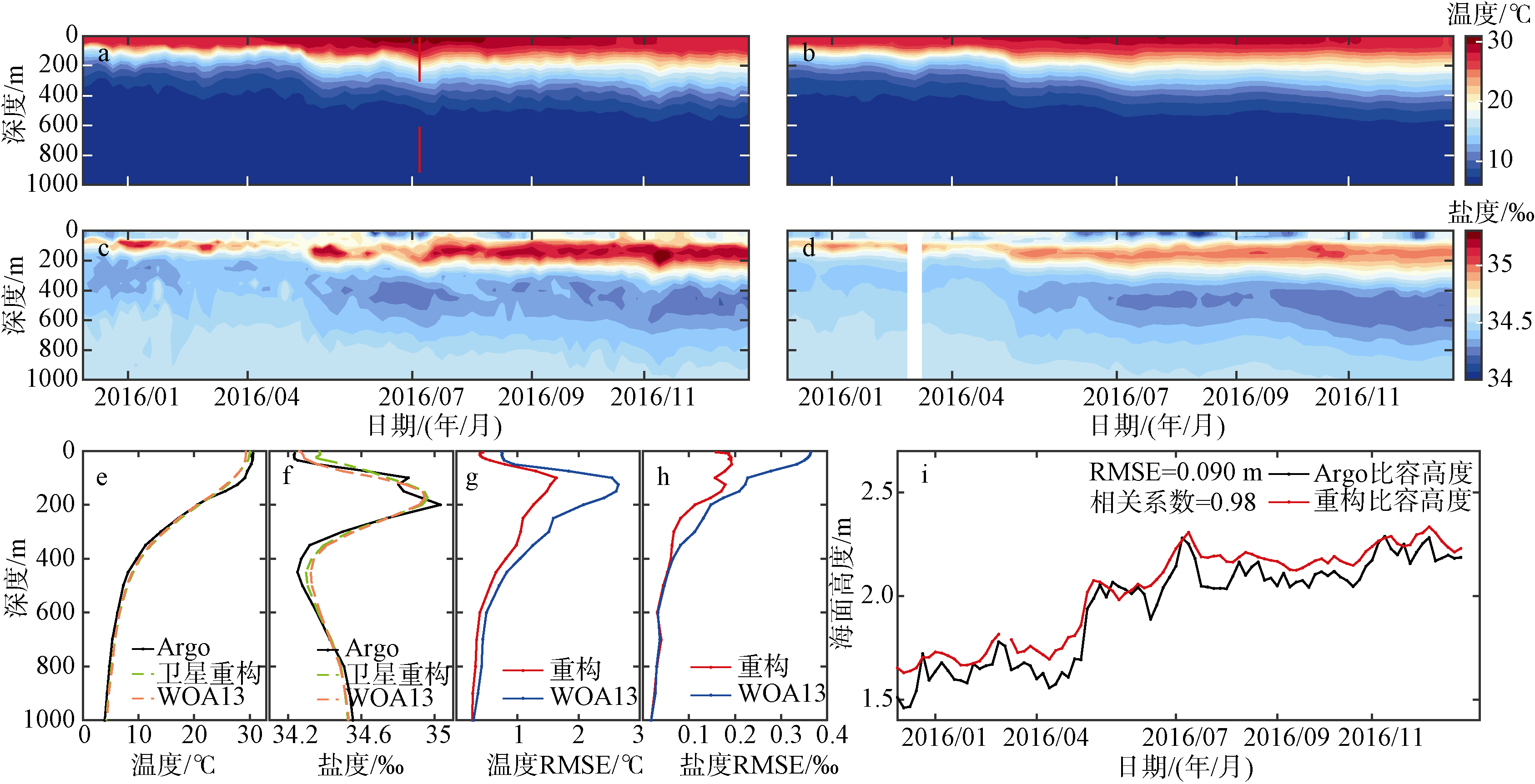
Fig. 13

Fig. 14
Temperature and salinity maps of all standard depths from 0 to 1000 m in each representative area. (a) North Pacific Ocean; (b) North Atlantic; (c) western equatorial Pacific; (d) eastern equatorial Pacific; (e) southern Indian Ocean; (f) Antarctic Ocean. Argo observation data (gray), satellite data reconstruction (green), and WOA climate state (blue)"
Fig. 14
Tab. 2
Vertical MRMSE of Argo observation data, satellite observation data reconstruction field and WOA climate state in each region"
| 卫星重构温度MRMSE/℃ | WOA13温度MRMSE/℃ | 卫星重构盐度MRMSE/‰ | WOA13盐度MRMSE/‰ | |
|---|---|---|---|---|
| 北太平洋 | 0.98 | 1.56 | 0.17 | 0.15 |
| 北大西洋 | 0.93 | 1.35 | 0.25 | 0.24 |
| 赤道西太 | 0.77 | 1.01 | 0.14 | 0.26 |
| 赤道东太 | 0.92 | 1.04 | 0.09 | 0.10 |
| 南印度洋 | 0.53 | 0.75 | 0.13 | 0.10 |
| 南大洋 | 0.48 | 0.70 | 0.17 | 0.10 |
| 平均 | 0.77±0.16 | 1.07±0.26 | 0.16±0.04 | 0.16±0.06 |
Tab. 2
| [1] | 鲍森亮, 张韧, 王辉赞, 等, 2018. 基于海表信息的海洋盐度剖面重构[C]// 第九届海洋强国战略论坛论文集. 北海: 海洋出版社: 206-215. (in Chinese) |
| [2] | 范良, 赵国忱, 苏运强, 2013. 果蝇算法优化的广义回归神经网络在变形监测预报的应用[J]. 测绘通报, (11): 87-89. |
| FAN LIANG, ZHAO GUOCHEN, SU YUNQIANG, 2013. Fruit fly optimization algorithm optimized general regression neural network in deformation monitoring and prediction[J]. Bulletin of Surveying and Mapping, (11): 87-89. (in Chinese with English abstract) | |
| [3] | 潘文超, 2011. 果蝇最佳化演算法: 最新演化式计算技术[M]. 台中: 沧海书局. (in Chinese) |
| [4] | 王喜冬, 韩桂军, 李威, 等, 2011. 利用卫星观测海面信息反演三维温度场[J]. 热带海洋学报, 30(6): 10-17. |
| WANG XIDONG, HAN GUIJUN, LI WEI, et al, 2011. Reconstruction of ocean temperature profile using satellite observations[J]. Journal of Tropical Oceanography, 30(6): 10-17. (in Chinese with English abstract) | |
| [5] | BALLABRERA-POY J, MOURRE B, GARCIA-LADONA E, et al, 2009. Linear and non-linear T-S models for the eastern North Atlantic from Argo data: Role of surface salinity observations[J]. Deep Sea Research Part Ⅰ: Oceanographic Research Papers, 56(10): 1605-1614. |
| [6] |
BAO SENLIANG, ZHANG REN, WANG HUIZAN, et al, 2019. Salinity profile estimation in the Pacific Ocean from satellite surface salinity observations[J]. Journal of Atmospheric and Oceanic Technology, 36(1): 53-68.
doi: 10.1175/JTECH-D-17-0226.1 |
| [7] | CHANG Y S, ROSATI A, ZHANG SHAOQING, 2011. A construction of pseudo salinity profiles for the global ocean: Method and evaluation[J]. Journal of Geophysical Research: Oceans, 116(C2): C02002. |
| [8] | CHEN ZHIQIANG, WANG XIDONG, LIU LEI, 2020. Reconstruction of three-dimensional ocean structure from sea surface data: An application of is QG method in the southwest Indian Ocean[J]. Journal of Geophysical Research: Oceans, 125(6): e2020JC016351. |
| [9] |
FUJII Y, KAMACHI M, 2003. A reconstruction of observed profiles in the sea east of Japan using vertical coupled temperature-salinity EOF modes[J]. Journal of Oceanography, 59(2): 173-186.
doi: 10.1023/A:1025539104750 |
| [10] |
GOES M, CHRISTOPHERSEN J, DONG SHENFU, et al, 2018. An updated estimate of salinity for the Atlantic Ocean sector using temperature-salinity relationships[J]. Journal of Atmospheric and Oceanic Technology, 35(9): 1771-1784.
doi: 10.1175/JTECH-D-18-0029.1 |
| [11] |
GUEYE M B, NIANG A, ARNAULT S, et al, 2014. Neural approach to inverting complex system: Application to ocean salinity profile estimation from surface parameters[J]. Computers and Geosciences, 72: 201-209.
doi: 10.1016/j.cageo.2014.07.012 |
| [12] |
GUINEHUT S, LE TRAON P Y, LARNICOL G, et al, 2004. Combining Argo and remote-sensing data to estimate the ocean three-dimensional temperature fields - a first approach based on simulated observations[J]. Journal of Marine Systems, 46(1-4): 85-98.
doi: 10.1016/j.jmarsys.2003.11.022 |
| [13] | HAN GUIJUN, ZHU JIANG, ZHOU GUANGQING, 2004. Salinity estimation using the T-S relation in the context of variational data assimilation[J]. Journal of Geophysical Research: Oceans, 109(C3): C03018. |
| [14] | HE ZIKANG, WANG XIDONG, WU XINRONG, et al, 2021. Projecting three-dimensional ocean thermohaline structure in the North Indian Ocean from the Satellite Sea surface data based on a variational method[J]. Journal of Geophysical Research: Oceans, 126(1): e2020JC016759. |
| [15] | HELBER R W, TOWNSEND T L, BARRON C N, et al, 2013. Validation test report for the improved synthetic ocean profile (ISOP) system, part Ⅰ: Synthetic profile methods and algorithm[R]. Naval Research Lab, Stennis Space Center, MS. Oceanography Div, 1-128. |
| [16] |
ISERN-FONTANET J, CHAPRON B, LAPEYRE G, et al, 2006. Potential use of microwave sea surface temperatures for the estimation of ocean currents[J]. Geophysical Research Letters, 33(24): L24608.
doi: 10.1029/2006GL027801 |
| [17] | ISERN-FONTANET J, LAPEYRE G, KLEIN P, et al, 2008. Three-dimensional reconstruction of oceanic mesoscale currents from surface information[J]. Journal of Geophysical Research: Oceans, 113(C9): C09005. |
| [18] |
KLEIN P, HUA B L, LAPEYRE G, et al, 2008. Upper ocean turbulence from high-resolution 3D simulations[J]. Journal of Physical Oceanography, 38(8): 1748-1763.
doi: 10.1175/2007JPO3773.1 |
| [19] |
NARDELLI B B, SANTOLERI R, 2004. Reconstructing synthetic profiles from surface data[J]. Journal of Atmospheric and Oceanic Technology, 21(4): 693-703.
doi: 10.1175/1520-0426(2004)021<0693:RSPFSD>2.0.CO;2 |
| [20] |
NARDELLI B B, COLELLA S, SANTOLERI R, et al, 2010. A re-analysis of Black Sea surface temperature[J]. Journal of Marine Systems, 79(1-2): 50-64.
doi: 10.1016/j.jmarsys.2009.07.001 |
| [21] |
SPECHT D F, 1991. A general regression neural network[J]. IEEE Transactions on Neural Networks, 2(6): 568-576.
doi: 10.1109/72.97934 |
| [22] |
WANG JINBO, FLIERL G R, LACASCE J H, et al, 2013. Reconstructing the Ocean’s interior from surface data[J]. Journal of Physical Oceanography, 43(8): 1611-1626.
doi: 10.1175/JPO-D-12-0204.1 |
| [23] | YANG TINGTING, CHEN ZHONGBIAO, HE YIJUN, 2015. A new method to retrieve salinity profiles from sea surface salinity observed by SMOS satellite[J]. Acta Oceanologica Sinica, 34(9): 85-93. |
| [1] | CHEN Shu, XU Hong, LU Shushen, Zhang Haiyang, MA Yazeng, LUO Jinxiong. The framework, reservoir characteristics and reef formation model of Miocene algal reef dolomite in the Xisha Islands* [J]. Journal of Tropical Oceanography, 2024, 43(2): 140-153. |
| [2] | HE Zikang, WANG Xidong, CHEN Zhiqiang, FAN Kaigui. Reconstructing salinity profile using temperature profile and sea surface salinity [J]. Journal of Tropical Oceanography, 2021, 40(6): 41-51. |
| [3] | WANG Xi-dong,HAN Gui-jun,LI Wei,QI Yi-quan . Reconstruction of ocean temperature profile using satellite observations [J]. Journal of Tropical Oceanography, 2011, 30(6): 10-17. |
|
||